
20 A Few More Things Before We Go
20.1 Adjusted \(R^2\)
Whenever we add terms to a model, even random stuff that has nothing to do with anything in the model, SSM will increase and RSS will decrease. This means that \(R^2\) will go up. That makes \(R^2\) difficult to use for the purpose of comparing two models if those two models have different numbers of terms: Is the larger model better just because it has more terms? Or is enough better – from the perspective of \(R^2\) – to make us think that is doing a better job of explaining the variation in our response variable?
An adjusted has been proposed to counteract this effect. The result is called adjusted \(R^2\) and it appears in the output produced by many statistical programs. Here is the definition:
\[ \mbox{adjusted-$R^2$} = 1 - \frac{ RSS / (n - k) }{SST / (n-1)} \]
where \(k\) is the number of coefficients in the model (including the intercept). Some things to notice:
adjusted-\(R^2 < R^2\)
This is because
\[ R^2 = \frac{SSM}{SST} = 1 - \frac{RSS}{SST} = 1 - \frac{ RSS / (n - 1) }{SST / (n-1)} \le 1 - \frac{ RSS / (n - k) }{SST / (n-1)} = \mbox{adjusted-$R^2$} \]
- adjusted-\(R^2\) is the ratio of two slopes (like the \(F\) statistic is, but it is two different slopes being compared). See Figure 20.1. In particular, adjusted-\(R^2\) will be negative whenever a model accounts for less variation in the response variable than a model with an equivalent number of random junk predictors would do on average.
The most important thing to understand is that the adjustment is intended to penalize models with more parameters. Why penalize larger, more complex models? They run the risk of over-fitting – reflecting the data too much and in ways that don’t reflect the population at large. This would certainly be the case if we use a random junk predictor since that random junk would not be replicated in the population – it was random and had nothing to do with the population. IF the new additions to our models can’t meet the threshold of “doing better than average random junk”, then it is hard to believe that any new patterns they discover will actually be reflected in the population.
Adjusted-\(R^2\) is not the only way to measure this. Several information criteria, like AIC and BIC, are also used to compare models. All of these methods penalize more complex models relative to less complex models to make it easier to do an apples-to-apples comparison. None of these is perfect, but all are better than using \(R^2\) without an adjustment.
20.2 Linear models by any other name…
If you have taken another statistics class or read papers describing statistical analyses, you might encounter things that seem somewhat familiar but not exactly the same as what we have seen through out this book. Many of these statistical procedures are equivalent to or very nearly equivalent to things we have done in this book, but done without the linear model framework that makes them all part of a common system.
This section will illustrate several of these “other methods” and show how they relate to various linear models that we have encountered. We focus on hypothesis tests primarily because (a) they are common in the literature and (b) confidence intervals look basically the same no matter what method was used to compute them – they are presented either as an upper and lower limit or as an estimate \(\pm\) margin of error.
For the first few of these we include that usual formula used to compute the test statistic. We won’t need to use these formulas – statistical software will take care of that. But they may be familiar to you from elsewhere.
In the literature, hypothesis tests are also presented succinctly. Usually all that is given is the test statistic, the p-value, and perhaps the degrees of freedom.
20.2.1 Notation used in this section
Y– quantitative responseX– quantitative explanatory variableA– binary response variable (2 levels)B– binary explanatory variable (2 levels)C– categorical explanatory variable (3 or more levels)
20.2.2 One-sample t (inference for 1 mean)
Formulas
The one-sample t-test is based on the following formulas for \(t\) and \(SE\):
- \(t = \frac{\overline{x} - \mu}{SE}; \qquad SE = \frac{s}{\sqrt{n}}\)
Equivalent model: lm(Y ~ 1)
This was our first model, the all-cases-the-same model.
Example Application: Body Temperature
As an example, let’s see whether the average body temperature for people is really 98.6 degrees Fahrenheit using a sample of 50 university students. Here’s is the relevant null hypothesis:
- \(H_0\): \(\mu = 98.6\).
Data Summary
| response | mean | sd |
|---|---|---|
| BodyTemp | 98.26 | 0.7653 |

Output comparison
One-sample \(t\)
The results of a one-sample t-test are usually presented something like this:
- \(t = -3.14\), \(p = 0.0029\), \(df = 49\).
This summary provides all of the critical information for the test very succinctly. We could also express the results by providing a confidence interval for the population mean (\(\mu\)).
Linear model
Here is the output from the linear model:
| Estimate | Std. Error | t value | Pr(>|t|) | |
|---|---|---|---|---|
| (Intercept) | 98.26 | 0.1082 | 907.9 | 3.318e-105 |
| Observations | Residual Std. Error | \(R^2\) | Adjusted \(R^2\) |
|---|---|---|---|
| 50 | 0.7653 | 0 | 0 |
Table 20.1: Summary of a linear model with no predictors.
20.2.3 Two-sample t (inference for comparing two means)
Formulas
The two-sample t-test is based on the following formulas for \(t\) and \(SE\):
- \(t = \frac{ \overline{x_1} - \overline{x_2}}{SE}\);
\(SE = \sqrt{ \frac{s_1^2}{n_1} + \frac{s_2^2}{n_2}}\)
Equivalent model: lm(Y ~ B)
Example Application: Body Temperature by Sex
Let’s compare body temperatures of men and women using the same data as in the previous example.
- \(H_0: \mu_{\mathrm{male}} = \mu_{\mathrm{female}}\); or, equivalently, \(H_0: \mu_{\mathrm{male}} - \mu_{\mathrm{female}} = 0\)
Data Summary
| response | Sex | mean | sd |
|---|---|---|---|
| BodyTemp | Female | 98.17 | 0.6755 |
| BodyTemp | Male | 98.35 | 0.8505 |
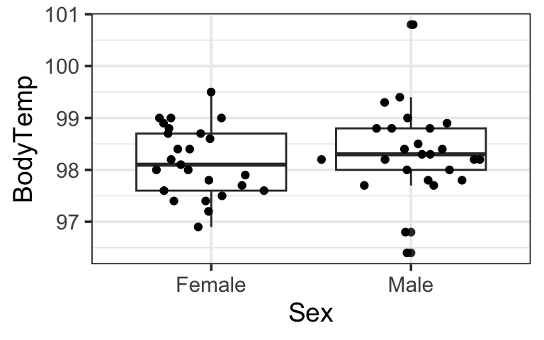
Output comparison
Two-sample t
- \(t = 0.81\), \(p = 0.422\), \(df = 45.66\)
Linear Model
The equivalent test is the test that the slope coefficient (\(\beta_1\)) is 0. We can find the results of this test in a traditional coefficients summary table or in an ANOVA table
| Estimate | Std. Error | t value | Pr(>|t|) | |
|---|---|---|---|---|
| (Intercept) | 98.17 | 0.1536 | 639.1 | 5.489e-96 |
| SexMale | 0.176 | 0.2172 | 0.8102 | 0.4218 |
| Sum Sq | Df | F value | Pr(>F) | |
|---|---|---|---|---|
| Sex | 0.3872 | 1 | 0.6564 | 0.4218 |
| Residuals | 28.31 | 48 | NA | NA |
Comments
There are 2 versions of the two-sample t procedures.
One of them assumes the two groups have equal variance (in the population) and is exactly equivalent to the linear model since the “slope” measures the difference between the means of the two groups.
The other is a bit more flexible and accounts for the situation where the two groups have different variances.
The degrees of freedom when using this approach is usually not an integer.
There is little reason not to use the more flexible version when working with t-tests in software. If the standard deviations are similar for each group, the two approaches will yield similar results, as the did in our example above.
If the standard deviations are quite different, we may need to ask whether we are really primarily interested in comparing the means.
The degrees of freedom for the 2-sample \(t\) is often not an integer. The value will be somewhere between
- one less than the size of the smaller group (i.e., degrees of freedom for smaller group),
- two less than the size of both groups combined (i.e., sum of the degrees of freedom for the two groups).
20.2.4 1-proportion
Tests and confidence intervals for one-proportion are often done using either the binomial test or a normal approximation to that test.
Formulas
The normal approximation to the binomial test is based on the following formulas for \(z\) and \(SE\):
- \(z = \frac{\hat p - p}{SE}; \qquad SE = \sqrt{\frac{p (1-p)}{n}}\)
Equivalent model: glm(A ~ 1, family = "binomial")
A logistic regression model with only an intercept term achieves the same thing. It also uses an approximate null distribution, so it is very similar to the normal approximation to the binomial test. The link value will be the log odds, which we can convert into a probability using the logistic transformation.
These lead to somewhat different intervals, since the logistic regression interval is symmetric on the log odds scale while the normal approximation to the binomial produces an interval that is symmetric on the probability scale.
Example: Testing a Coin
Suppose we flip a coin 100 times had observe 58 heads. Is that enough to lead to concern about whether the coin is fair?
- \(H_0\): \(p = 0.50\).
Output comparison
Binomial test
- \(\hat p = 0.58\), \(p = 0.1332\)
Normal approximation to the binomial test
- without “continuity correction”: \(\chi^2 = 2.56\) (\(z = 1.6\)); \(p = 0.1096\), (\(df = 1\))
- with “continuity correction”: \(\chi^2 = 2.25\) (\(z = 1.5\)); \(p = 0.1336\), (\(df = 1\))
Logistic regression
| term | Estimate | Std Error | t | p-value |
|---|---|---|---|---|
| (Intercept) | 0.323 | 0.203 | 1.59 | 0.1111 |
Comments
One proportion tests may be presented using either a \(z\) (normal) or a Chi-squared statistic. These are equivalent. The Chi-squared statistic is obtained by squaring the \(z\) statistic. The degrees of freedom for the Chi-squared distribution in this situation is 1.
20.2.5 Difference between two proportions
There are several ways you might see two proportions compared.
- A two-proportion test (based on normal approximations)
- A Chi-squared test for a 2-by-2 table
- Fisher’s exact test
Formulas
The normal approximation leads to the following formulas for \(z\) and \(SE\):
- \(z = \frac{(\hat p_1 - \hat p_2) - (p_1 - p_2)}{SE}; \qquad SE = \sqrt{\frac{p_1 (1-p_1)}{n_1} + \frac{p_2 (1-p_2)}{n_2}}\)
The Chi-squared test is based on a different test statistic that has an approximately Chi-squared distribution, and Fisher’s exact test is based on hypergeometric distributions.
Equivalent model: glm(A ~ B, family = "binomial")
The linear modeling approach here is to fit a logistic regression model with a binary predictor. The link values are the log odds for each group, which can be converted to proportions using the logistic transformation.
Example: Pain Relief
Suppose we are testing pain relief medication to see if it performs better than a placebo. In the study, 150 people were randomly assigned to take one of the two, without knowing which pill they were given and asked to report if they experienced pain relief.
Data Summary
| relief | Medication | Placebo | Total |
|---|---|---|---|
| No | 39 | 54 | 93 |
| Yes | 36 | 21 | 57 |
| Total | 75 | 75 | 150 |
- \(H_0\): the proportion of people experience pain relief is the same for the medication and the placebo.
Output comparison
Chi-squared test or 2-proportion test
- \(\chi^2 = 5.5461\), \(df = 1\), \(p = 0.01852\)
Fisher’s test
- odds ratio \(= 0.424\), \(p = 0.01815\)
Logistic regression
In this situation, we can get the desired p-value either from the summary table or from the ANOVA table. The two approaches use slightly different null distribution approximations, so the p-values are not identical, even though they are testing the same null hypothesis.
| Estimate | Std. Error | z value | Pr(>|z|) | |
|---|---|---|---|---|
| (Intercept) | -0.08004 | 0.2311 | -0.3463 | 0.7291 |
| treatmentPlacebo | -0.8644 | 0.3458 | -2.5 | 0.01242 |
| LR Chisq | Df | Pr(>Chisq) | |
|---|---|---|---|
| treatment | 6.424 | 1 | 0.01126 |
Table 20.3: Testing the difference between two proportions using logistic regression.
20.2.6 Inference for 2-way tables: Chi-squared tests
Chi-squared tests can also be used for tables that are larger than 2-by-2.
- \(H_0:\) There is no association between two categorical variables (in the population).
Equivalent model: lm(Y ~ B) or lm(Y ~ C)
As long as one of the two categorical variables has only 2 levels, we can use logistic regression to test the same null hypothesis. The null hypothesis of the model utility test is equivalent to the null hypothesis for the Chi-squared test: no association between the explanatory and response variables.
Example: Bank Customers
A local bank records the age distribution of customers coming to two branches to see how they compare:
- \(H_0\): The age distributions are the same at both branches.
Data Summary
| <30 | 30-55 | >55 | Total | |
|---|---|---|---|---|
| A | 20 | 50 | 40 | 110 |
| B | 30 | 40 | 20 | 90 |
| Total | 50 | 90 | 60 | 200 |
Output comparison:
Chi-squared test
- \(\chi^2 = 7.8563\), \(df = 2\), \(p = 0.0197\).
Logistic regression
The ANOVA table gives essentially the same results.
| LR Chisq | Df | Pr(>Chisq) | |
|---|---|---|---|
| age | 7.92 | 2 | 0.01907 |
Comments
There are two reasons to prefer the logistic regression to the Chi-squared approach.
Both methods use an approximate null distribution, but the one used by logistic regression is considered a better approximation.
Logistic regression provides a natural way to ask follow up questions about which proportions differ from which others.
20.3 Why linear models?
This book adopts a modeling approach to statistics for several reasons.
The linear model approach places many things into a common framework.
As seen above, situations that can be handled by 1- and 2-sample t-tests or by methods for 1 or 2 prportions, can just as easily be analysed using a linear model. The advantage of the linear model approach is that all the different analyses are part of a common frameowrk. Once that framework is learned, a wide variety of situations can be analysed.
It is more readily generalizable.
The traditional approach that focuses on situataions with one or two variables and provides no tools to deal with covariates. But most statistical analyses includes covariates. The linear model approach is very flexible and allows for adding additional covariates, interaction, transformations, etc.
Linear models are heavily used in many domain disciplines.
As one example of the increasing trend toward using multiple linear regression (linear models with more than a single explanatory variable), (Horton and Switzer 2005) did a survey of statistical methods used in the New England Journal of Medicine. In 1989, only 14% of the articles surveyed used mutliple regression, but by 2004-05, that had increased to 51%. Additional papers included methods like 1-way ANOVA or t-tests that could be done using the linear model framework. Only 20% of 2004-05 articles included only simple methods like t-tests and 1-way ANOVA.
Comments
These two methods are exactly equivalent. The same test-statistics, p-values, and confidence intervals are produced using either method.
Note that to test our desired the null hypothesis using the linear model output we must compute our test statistic and p-value using the estimate and standard error in the summary table. (The test presented in the summary table is for \(H_0: \beta_1 = 0\); we have very strong evidence against the hypothesis that the mean body temperature is 0 degrees Fahrenheit, but that isn’t an interesting result.) The p-value is computed using the t-distribution with \(n - 1 = 49\) degrees of freedom.
\[ t = \frac{98.26 - 98.6}{0.1082} = -3.142 \]