5 Confidence Intervals
Most of the time we are not directly interested in our data but in what our data can tell us about something bigger or more general. We collect data on a company and its past stock performance to predict its future performance. We gather a sample of likely voters in hopes of predicting the outcome of an election. Each month the US Bereau of Labor Statistics (BLS) surveys approximately 60,000 households to gather the data it uses to estimate the unemployment rate in the entire country (and in various subgroups within the population).
It’s easy enough to calculate the mean or median within groups, especially using software. Less obvious to those starting out in statistics is the idea that a quantity such as the mean or median itself has limited precision as an estimate of that value in the population. This isn’t a matter of the calculation itself. If the calculation has been done correctly, the resulting quantity is exactly right for the data at hand. The limited precision arises from the sampling process that was used to collect the data. The exact mean or median relates to the particular sample you have collected. Had you collected a different sample, it’s likely that you would have gotten a somewhat different value for the quantities you calculate. This variability of a statistic from sample to sample from the same population is called sampling variability. One purpose of statistical inference is to quantify sampling variability, that is, to measure how different these “somewhat different values” might be. When there is a lot of sampling variability, then our estimate is not very precise – it might differ from the value we are trying to estimate by a considerable amount. But if sampling variability is low, then it is likely that the estimate computed from our sample is quite close to the value we are trying to estimate in the population. The BLS needs a large sample each month because they need to estimate the unemployment rate with high precision in order to detect changes and trends early.
5.1 The Sampling Distribution
An estimate of the limits to precision that stem from sampling variability can be made by simulating the sampling process itself. To illustrate, consider again the data in the TenMileRace table. These data give the running times of all 12,302 participants in a ten-mile long running race held in Washington, DC in March 2008.
Suppose want to describe how women’s running times differ from men’s. In this case, we have data for every runner (a census), but suppose we did not. Suppose we only had a sample of size n = 200.
Here are are the groupwise means calculated for one such sample:
| sex | mean running time (minutes) |
|---|---|
| F | 103.6 |
| M | 87.9 |
How well could we estimate the mean running times for all men and for all women from this sample? Let’s try another sample of size n = 200 and see how the estimate compare.
| sex | mean running time (minutes) |
|---|---|
| F | 101.8 |
| M | 91.5 |
Each new random sample of size n = 200 will generate new estimates – they will all be somewhat different from the others. But how different will they be?
The sampling distribution describes how different the statistics computed from different random samples will be. The word “random” is very important here. Random sampling helps to ensure that the sample is representative of the population and that we have a way to quantify the sampling variability.
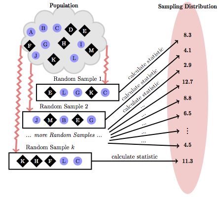
The process of generating the sampling distribution is shown in Figure 5.1. Take a random sample from the sampling frame and calculate the statistic of interest. (In this case, that’s the mean running time for men and for women.) Do this many times. Because of the random sampling process, you’ll get somewhat different results each time. The spread of those results indicates the limited precision that arises due to sampling variability.
Historically, the sampling distribution was approximated using algebraic techniques. But it’s perfectly feasible to use the computer to repeat the process of random sampling many times and to generate the sampling distribution through a simulation.

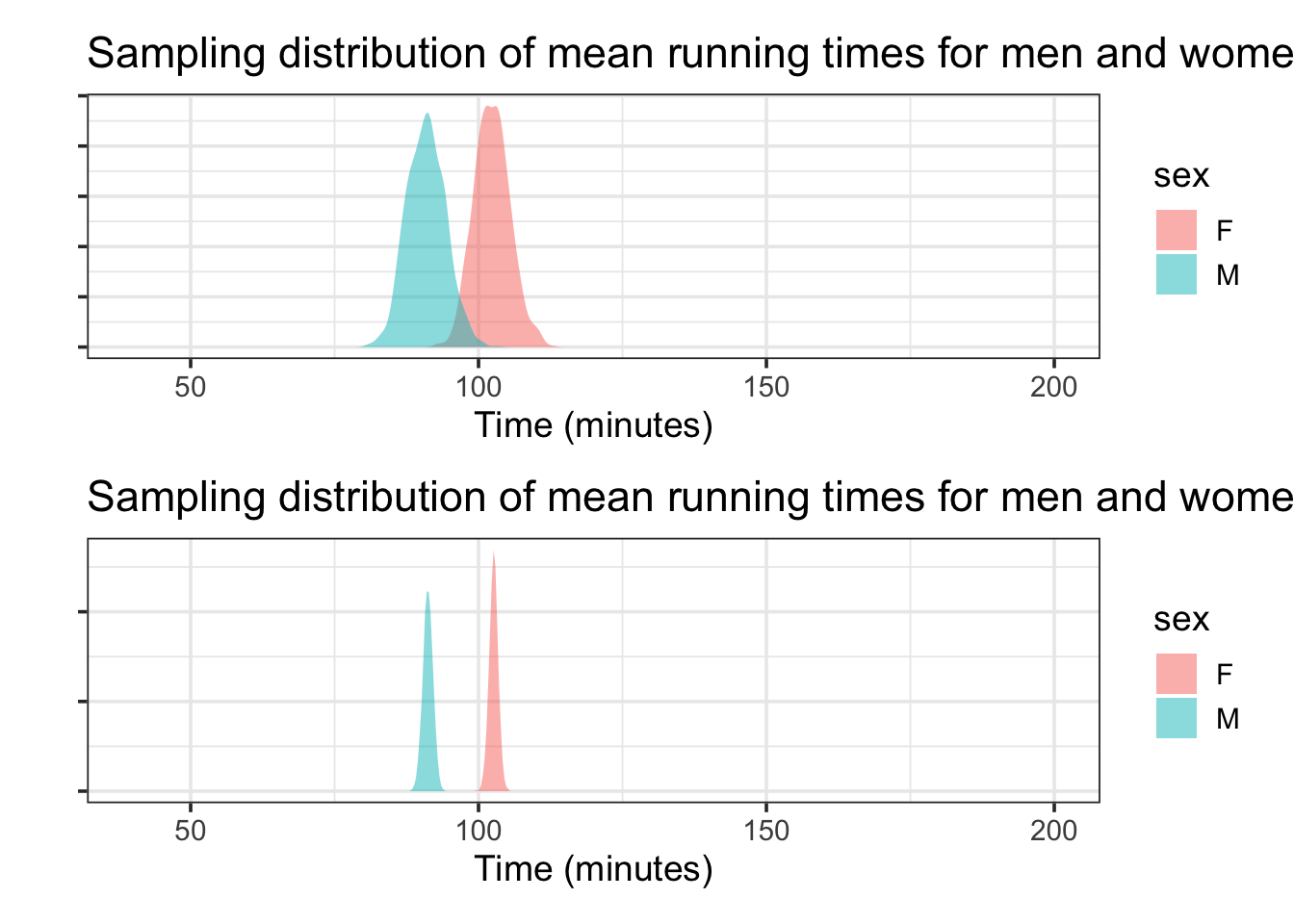
The sampling distribution depends on both the data and on the statistic being calculated. Figure 5.2 shows both the distribution of individual running times – the data themselves! – and the sampling distribution for the means of men’s and women’s running time for a sample of size n = 200.
Notice that the sampling distribution of the mean running times for n = 200 is much narrower than the individual data. That’s because, in taking the mean, the fast running times tend to cancel out the slow running times.
One way to quantify the precision of a measurement is called a confidence interval. This is commonly written in either of two equivalent ways:
- Plus-or-minus format: 87.9 ± 3.1 minutes with 95% confidence.
- Range format: 84.8 to 91.1 minutes with 95% confidence.
Our goal for this chapter is to understand how these confidence intervals are computed and what they tell us.
If the sample size had been smaller, the confidence interval would be wider; that is, smaller samples result in less precise estimates. Similarly, larger samples produce narrower confidence intervals. Figure 5.3 shows the sampling distributions for the mean of the running times for samples of size n = 50 and n = 800. Notice that when n = 50, the sampling distributions are wider and when n = 800 the sampling distributions are narrower. We can make more precise estimates from larger samples than from smaller samples.
The logic of sampling distributions and confidence intervals applies to any statistic calculated from a sample, not just the means used in these examples but also proportions, medians, standard deviations, inter-quartile intervals, etc.
In keeping with the Pythagorean principle, it’s the square of the precision that behaves in a simple way, just as it’s the square of triangle edge lengths that add up in the Pythagorean relationship. As a rule, the square width of the sampling distribution scales with 1/\(n\), that is,
\[\mbox{width}^2 \propto \frac{1}{n}.\] Taking square roots leads to the simple relationship of width with \(n\):
\[\mbox{width} \propto \frac{1}{\sqrt{n}}.\]
To improve your precision by a factor of two, you will need 4 times as much data. For ten times better precision, you’ll need 100 times as much data.
5.2 The Resampling Distribution & Bootstrapping
The construction of the sampling distribution by repeatedly collecting new samples from the population is theoretically sound but has a severe practical short-coming: It’s hard enough to collect a single sample of size n, but infeasible to repeat that work multiple times to sketch out the sampling distribution. For almost all practical work, we will need to estimate the properties of the sampling distribution from your single sample of size n.
There are generally two approaches to discovering properties of the sampling distribution.
Theoretical Methods: Sometimes mathematics allows us to derive properties of the sampling distribution.
These derivations are generally well beyond the scope of this book, but for simple study designs, the resulting formulas are often pretty reasonable – even for humans. And in more complicated situtations, these formulas can be programmed into statistical software.
These mathematical results typically rely on making some simplifying assumptions about the population. But as long as the assumptions are reasonably close to reality, these methods work well. (Checking that this is the case is an important part of using these methods.)
Simulation-based Methods: Simulations can help us extract information about the sampling distribution from our sample.
These methods go by names like bootstrapping or resampling. The word bootstrapping is drawn from the phrase, “to pull oneself up by one’s bootstraps”, said of people who improve through their own efforts, without assistance.
To carry out a statistical bootstrap, you substitute your sample in place of the overall sampling frame, and draw many new samples from the original sample (using a computer to automate the work). The idea is that if the original sample is a good representation of the population, then these bootstrap samples should give us a good representation of the sampling distribution.
5.2.1 Resampling
The sample is already in hand, in the form of a data frame, so it’s easy to draw cases from it. Such new samples, taken from your original sample, not from the population, are called bootstrap samples or resamples. These are samples drawn from the original sample. :
Figure 5.4 illustrates how resampling works. There is just one sample drawn – with actual labor and expense – from the real population. Thereafter, the sample itself is used as a stand-in for the population and new samples are drawn from the sample.
Will such resamples capture the sampling variation that would be expected if you were genuinely drawing new samples from the population? An objection might come to mind: If you draw \(n\) cases out of a sample consisting of \(n\) cases, the resample will look exactly like the sample itself. There will be no variation from resample to resample. This problem is easily overcome by sampling with replacement.
Whenever a case is drawn from the sample to put in a resample, the case is put back so that it is available to be used again. This is not something you would do when collecting the original sample; in sampling (as opposed to resampling) you don’t use a case more than once.

The resamples in Figure 5.4 may seem a bit odd. They often repeat cases and omit cases. And, of course, any case in the population that was not included in the sample cannot be included in any of the resamples. Even so, the resamples do the job: they simulate sample to sample variation in a way that let’s us estimate the precision of the estimates produced by our original sample. Those estimates will typically be parameters of our model: group means, or the difference bewtween two group means, or some other quantity related to coefficients of a model.
5.2.2 The Resampling Distribution
The resampling distribution is the distribution of some statistic computed from each of our resamples. If we are interested in the mean running time of women, then we will calculate the mean running time of the women in many resamples. The distribution of these reseampled means is the resampling distribution.
It’s important to emphasize what the resamples can and cannot do:
Resampling doesn’t make estimates any more precise, it only helps us estimate the sampling variability.
The resamples merely show what the sampling distribution would look like if the population looked like our sample. The center of the resampling distribution is generally not aligned exactly with the center of the population-based sampling distribution – it will tend to be centered at the center of the sample. However, in practice, the width (ie, standard deviation) of the resampling distribution is a good match to the width of the sampling distribution. In many situations, the resampling distribution is adequate for the purpose of finding standard errors, margins of error, and confidence intervals.
As an example, let’s look at the resampling distributions that arise from the women’s running times in our two samples above.

Notice that the centers of the two resampling distributions are a bit different, but the shape and spread in each is nearly identical. This is our estimate for the sampling variability. The centers of the two sampling distributions are near the means from each of the two samples. This does not give us any new information – we already knew the centers of the samples.
5.2.3 Confidence intervals from resampling distributions
So how do we get a confidence interval from a resampling distribution? It turns out that there are several different ways to do it. For now, we will focus on two of the simplest methods
Coverage intervals as confidence intervals
The resampling distribution indicates the amount of variation in our statistic from sample to sample. If most of the boostrap statistics are close to the original estimate, then we have reason to believe that our original estimate is likely close to the quantity we are estimating. We just need to quantify most and close.
One way to do this is to take a coverage interval for the resampling distribution. A 95% coverage interval of a resampling distribution becomes our estimate for a 95% confidence interval for the quantity being estimated.
Here is an example using 1000 resamples. To get the 95% coverage interval, we remove the 25 largest and 25 smallest resample means.
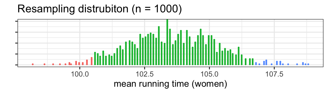
The resulting interval is (100.5, 106.7).
Bootstrap standard error intervals
The bootstrap standard error method only works well if the resampling distribution is roughly symmetric and bell-shaped, like the one in our example. In this case, the portion of the distribution that extends from 2 standard deviations below the mean to two standard deviations above the mean is approximately 95%. So we can approximate the 95% coverage interval as
\[ \mbox{sample statistic} \pm 2 * SE \]
where \(SE\) (standard error) is the standard deviation of the resampling distribution.
In our example, the mean running time of women in our original sample is 103.6, and \(SE = 1.6\), so our 95% confidence interval can be written in the following ways:
\[ \begin{aligned} 103.6 &\pm 2 \cdot 1.6\\ 103.6 &\pm 3.2\\ ( 100.4 &, 106.8 ) \end{aligned} \]
The two approaches give quite similar results. The first method is more flexible since it can adjust better for resampling distributions that are skewed or that are flatter or more peaked than the “normal” bell-shape. The main reason for presenting the boostrap standard error method is that it closely resembles the theoretical methods we will see later. Those methods using mathematics instead of simulations to estimate the standard error. So many confidence intervals will have the form
\[ \mbox{sample estimate} \pm (\mbox{some number}) \cdot SE \] where “some number” depends on the level of confidence and the shape of the (re)sampling distribution. That number is typically close to 2 for the types of models we will encounter.
Both methods can be improved by taking more advantage of the information in our bootstrap distribution. But these simple methods will be good enough to help us understand the idea of a confidence interval and they work quite well for the types of models that we will see.
5.3 Interpreting Confidence Intervals
Creating confidence intervals is relatively easy. We have three methods:
Use a coverage interval of a resampling distribution distribution.
\(\mbox{sample estimate} \pm (\mbox{some number}) \cdot SE\)
- SE can be estimated using the standard deviation of a resampling distribution.
- SE can be estimated using a mathematically derived formula.
Intuitively, a confidence interval can be thought of as a plausible set of values for the parameter being estimated. That’s good as far as it goes, but what does plausible really mean, and how do we quantify pluasibility?
5.3.1 Confidence level and coverage rates
Each confidence interval that we produce is either “correct” (it contains the parameter being estimated) or “incorrect” (it does not contain the parameter). The percent of confidence intervals that are correct using a given method is called the coverage rate. The goal of a confidence interval method is to have the coverage rate be equal to the confidence level. For example, the goal of a 95% confidence interval method is to be “correct” 95% of the time. Rather than calling these intervals “correct”, statisticians say that such intervals cover the parameter being estimated.
This is tricky because we only have one sample and one confidence interval, and we won’t know whether it covers or not. But we can study the method used to see whether the method covers with (approximately) the stated confidence level.
All three of our methods are trying to achieve the stated coverage rate.
5.3.2 Confidence level is arbitrary
It is traditional to use a 95% confidence level. Changing the confidence level to 90% or 99% doesn’t change the precision of our estimate, only the particular way we are describing that precision. In this sense, the choice is arbitrary.
Here is an anology. Suppose you decide to take up archery. You are not particularly good at archery, so you decide to get a bigger target so you can hit it more often. You will indeed hit the target more often by doing this, but you won’t be a better archer. All you have done is change the way you are measuring how precise you are. Confidence levels are similar. 99% confidence interval will cover more often because the target (interval) is larger. 90% confidence intervals will cover less often because the target (interval) is smaller. But both are telling us something about the same underlying precision of the estimate.
For archery competition, standard distances and target sizes have been established. This makes it easier to compare results across events. The 95% confidence level is similar. By using it consistently, it is easier to compare results from one dataset to another.
The 95% confidence level is standard in contemporary science; it’s a convention. For that reason alone, it is a good idea to use 95% so that the people reading your work will tend to interpret things correctly. The choice of 95% is conventional and uncontroversial, but sometimes people choose – for good reasons or bad – to use another level such as 99% or 90%. Just remember that the choice of confidence level doesn not effect the underlying precision of the estimate, it is just another way to describe the same level of precision.
One difference between archery and confidence intervals is that when constructing a confidence interval, we never know whether it has covered. This is different from archery, where we can always tell whether we have hit the target. The interesting thing about confidence interval methods is that we can determine the coverage rates of a method even though we never know which individual intervals cover and which do not.
You might wonder why statisticians to don’t use a confidence level of 100%. Surely it would be nice to be correct every time! But a 100% confidence interval would be too broad to be useful. In theory, 100% confidence intervals tend to look like -∞ to ∞. No information there! Complete confidence comes at the cost of complete ignorance.
The vocabulary of “confidence interval” and “confidence level” can be a little misleading. Confidence in everyday meaning is largely subjective, and you often hear of people being “over confident” or “lacking self-confidence.” It might be better if a term like “sampling precision interval” were used. In some fields, the term “error bar” is used informally, although “error” itself may have nothing to do with it; the precision stems from sampling variation.
5.3.3 Confidence intervals are not about individuals
Confidence intervals are easy to construct, whether by bootstrapping or other techniques. The are also very easy to misinterpret. One of the most common misinterpretations is to confuse the statement of the confidence interval with a statement about the individuals in the sample. For example, consider the confidence interval for the running times of men and women. Using our first sample of 200 runners (Table 5.1), we obtain a 95% confidence interval for the mean time of women of \(103.6 \pm 3.3\) and for men we get \(87.9 \pm 3.1\).
Importantly, this does not mean that most men and women have times that fall within these intervals. We can easily see that when we look at Figure 5.2 (top).
Confidence intervals are often mistakenly interpreted as if they were telling us something about the distribution of individuals in the population. But confidence intervals are not intended to tell us about the distribution of some value in the population, they are intended to tell us about the precision of some estimate we are making using a sample. There is a lot of evidence in our sample of 200 Cherry-Blossom running times to suggest that the mean running time for men is faster than for women. But many individual women run faster than individual men. A narrow confidence interval tells us how precisely we are estimating the mean running time using our sample. But the confidence interval does not tell us how much a typical individual differs from the mean.
5.3.4 The goal of a confidence interval is to cover the parameter, not other estimates
A 95% confidence interval always contains the sample estimate. 95% of 95% confidence intervals contain the parameter being estimated. It is tempting the think, “If I repeated my study with a different random sample, then there is a 95% chance that the estimate from the new sample will be within the 95% confidence interval produced from the first sample.” But that statement isn’t correct mathematically. The percentage will be less than 95% since we have two sources of variability: Neither sample perfectly estimates the parameter.
5.3.5 Confidence intervals are about precision of estimates
Treat the confidence interval just as an indication of the precision of the measurement. If you do a study that finds a statistic of 17 ± 6 and someone else does a study that gives 23 ± 5, then there is little reason to think that the two studies are inconsistent. On the other hand, if your study gives 17 ± 2 and the other study is 23 ± 1, then something seems to be going on; you have a genuine disagreement on your hands.
5.3.6 Confidence intervals from census data
Recall the distinction between a sample and a census. A census involves every member of the population, whereas a sample is a subset of the population.
The logic of statistical inference applies to samples and is based on the variation introduced by the sampling process itself. Each possible sample is somewhat different from other possible samples. The techniques of inference provide a means to quantify “somewhat” and a standard format for communicating the imprecision that necessarily results from the sampling process.
But what if you are working with the population: a census not just a sample? For instance, the employment termination data is based on every employee at the firm, not a random sample.
One point of view is that statistical inference for a census is meaningless: the population is regarded as fixed and non random, so the population parameters are also fixed. It’s sampling from the population that introduces random variation.
A different view, perhaps more pragmatic, considers the population itself as a hypothetically random draw from some abstract set of possible populations. For instance, in the census data, the particular set of employees was influenced by a host of unknown random factors: someone had a particularly up or down day when being interviewed, an employee became disabled or had some other life-changing event.
Similarly, when a unvirsity computes the grade point average or a student, they are using data from all of the courses a student has taken – a census. Since there is no sampling, there is no sampling variability to estimate and the the idea of sampling precision doesn’t make sense. On the other hand, it’s reasonable to consider that course choice and grades are influenced by random factors: schedule conflicts, what your friend decided to take, which instructor was assigned, which particular questions were on the final exam, and so on. So you can thinkg of a student’s actual grade point average as an approximation to what it might have been under all possible conditions, not just the conditions that actually occurred.
You can certainly calculate the quantities of statistical inference from the complete population, using the internal, case-by-case variation as a stand-in for the hypothetical random factors that influenced each case in the population. Interpreting confidence intervals from populations in the same way as confidence intervals from a sample can provide a useful indication of the strength of evidence, and indeed is recognized by courts when dealing with claims of employment discrimination. It does, however, rely on an untestable hypothesis about internal variation, which might not always be true.
Compare, for example, two possible extreme scenarios of course choice and grades. In one, students select courses on their own from a large set of possibilities. In the other scenario, every student takes exactly the same sequence of courses from the same instructors. In the first, it’s reasonable to calculate a confidence interval on the grade-point average and use this interval to compare the performance of two students. In the second scenario, since the students have all been in exactly the same situation, there might not be a good justification for constructing a confidence interval as if the data were from a random sample. For instance, there might be substantial internal variation because different instructors have different grading standards. But since every student had the same set of instructors, that variation shouldn’t be included in estimating sampling variation and confidence intervals.
The reality, for courses and grades at least, is usually somewhere between the two scenarios. The modeling techniques described in later chapters provide an approach for pulling apart the various sources of variation, rather than ascribing all of it to randomness and including all of it in the calculation of confidence intervals.
5.4 How many digits
Computers often report far more digits than are valuable or important. So how do we know how many digits to report? Confidence intervals can guide us here.
The margin of error should usually be reported to 1 or 2 significant digits. That is the first 1 or two digits that are not 0.
The estimate and lower and upper bounds of the interval should be reported to the same decimal place as the margin of error.
Why is this? Let’s suppose our estimate is \(27.545671\) and our margin of error (reporting two significant digits) is \(\pm 0.32\). That means that values like \(27.4\) or \(27.8\) are plausible. But values like \(27.1\) or \(27.9\) are not. Reporting the thousandths or ten thousandths make a lot of sense when we are not even sure about the tenths digit. Reporting to tenths:
\[ 27.5 \pm 0.3 \]
or to hundredths
\[ 27.55 \pm 0.32 \]
are reasonable descriptions of what we know from our data.
You should do your rounding after doing all of your calculations, not while you are doing the arithmetic. Rounding early can magnify the imprecision. So let the computer compute all those digist for you, then round appropriately at the end when reporting to a human.