| Intercept | age | sexM |
|---|---|---|
| 5339 | 16.89 | -726.6 |
12 Confidence in Models
To know one’s ignorance is the best part of knowledge. – Lao-Tsu (6th century BC), Chinese philosopher
Doubt is not a pleasant condition, but certainty is an absurd one. – Voltaire (1694-1778), French writer and philosopher
12.1 Linear Models and and Randomness
If you are a skilled modeler, you try to arrange things so that your model coefficients are random numbers.
That statement may sound silly, but before you jump to conclusions it’s important to understand where the randomness comes from and why it’s a good thing. Then you can use the tools in the previous two chapters to deal with the randomness and interpret it.
Recall the steps in building a statistical model:
- Collect data. This is the hardest part, often involving great effort and expense.
- Design your model, choosing the response variable, the explanatory variables, and the model terms. (It’s sensible to have the design in mind before you collect your data, so you know what data are needed.)
- Fit the model design to your data.
Step (3) is entirely deterministic. Given the model design and the data to which the model is to be fitted, fitting is an automatic process that will give the same results every time and on every computer. There is no randomness there. (There is some choice in choosing which to remove from a set of vectors containing redundancy, but that is a choice, not randomness. In any event, the fitted model values are not affected by this choice.)
Step (2) appears, at first glance, to leave space for chance. After all, when explanatory terms are collinear, as they often are, the fitted coefficients on any term can depend strongly on which other terms have been included in the model. The coefficients depend on the modeler’s choices. But this means only that the coefficients reflect the beliefs of the modeler. If those beliefs aren’t random, then the randomness of coefficients doesn’t stem from the modeler.
It’s step (1) that introduces the randomness. In collecting data, the sample cases are selected from a population. As described in Chapter 2, it’s advantageous to make a random selection from the population; this helps to make the sample representative of the population.
Saying something is random means that it is uncertain, that if the process were repeated again the result might be different. When a sample is selected at random, the particular sample that is produced is just one of a set of possibilities. One can imagine other possibilities that might have come about from the luck of the draw.
Insofar as the sample is random, the coefficients that come from fitting the model design to the sample are also random. The randomness of model coefficients means that the coefficients that come from a model design fitted to any particular data set are not likely to be an exact match to what you would get if the model design were fitted to the entire population. After all, the randomly selected sample is unlikely to be an exact match to the entire population.
It’s helpful to know how close the results from the sample are to what would have been obtained if the sample had been the entire population. Ultimately, the only way to know this for sure is to create a sample that is the entire population. Usually this is impractical and often it is impossible.
As described in Chapter 5, there is an approach that will give insight, even if it does not give certainty. To start, imagine that the sample were actually a census: a sample that contains the entire population. Repeating the study with a new sample would give exactly the same result because the new sample would be the same as the old one; it’s the same population.
When the sample is not the entire population, repeating the study won’t give the same result every time because the sample will include different members of the population. If the results vary wildly from one repetition to another, you have reason to think that the results are not a reliable indication of the population. If the results vary only a small amount from one repetition to another, then there’s reason to think that you have closely approximated the results that you would have gotten if the sample had been the entire population. The repeatability of the process indicates how well the modeler knows the coefficients, or, in a word, the precision of the coefficients.
Knowing the precision of coefficients is key in drawing conclusions from them. Consider Galton’s problem in studying whether height is a heritable trait. Had Galton known about modeling, he might have constructed a model like height ~ 1 +mother + father + sex. A relationship between the mother's height and her child's height should show up in the coefficient onmother`. If there is a relationship, that coefficient should be non-zero.
Fitting the model to Galton’s data, the coefficient is 0.32. Is this non-zero? Yes, for this particular set of data. But how might it have been different if Galton repeated his sampling, selecting a new set of cases from the population? How precise is the coefficient? Until this is known, it’s mere bravado to say that a result of 0.32 means anything.
This chapter introduces methods that can be used to estimate the precision of coefficients from data. A standard format for presenting this estimation is the confidence interval. For instance, from Galton’s data, the estimated coefficient on mother is 0.32 ± 0.06, giving confidence that a different sample would also show a non-zero coefficient.
It’s important to contrast precision with accuracy. Precision is about repeatability. Accuracy is about how the result matches the real world. Ultimately, accuracy is what the modeler wants. A major reason to introduce modeling techniques beyond the simple groupwise models of Chapter 4 is to enable you to account for the multiple factors that shape outcomes. But the results of a model always depend on the choices the modeler makes, e.g., which explanatory variables to include, how to choose a sample, etc. The results can be accurate only if the modeler makes good choices. Knowing whether this is the case depends on knowing how the world really works, and this is what you are seeking to find out in the first place. Accuracy is elusive knowledge. Precision will have to suffice.
12.2 Model Coefficients and Sampling Distributions
The same principles of sampling and re-sampling distributions introduced in Chapter 5 can be used to find confidence intervals on model coefficients.
To illustrate, consider the TenMileRace dataset (in the mosaicData package). This is a census containing the running times for all 8636 registered participants in the Cherry Blossom Ten Mile race held in Washington, D.C. in April 2005.
The variable net records the start-line to finish-line time of each runner. There are also variables age and sex. Any model would do to illustrate the sampling distribution. Let’s consider net ~ 1 + age + sex.
Just for reference, here are the coefficients when the model is fit to the entire population:
The coefficients indicate that,
runners who are one year older tend to take about 17 seconds longer to run the 10 miles;
men run about 726 seconds faster than women (of the same age).
Of course, if you knew the coefficients that fit the whole population, you would hardly need to collect a sample! But the purpose here is to demonstrate the effects of a random sampling process. The table below gives the coefficients from several sampling draws; each sample has \(n=100\) cases randomly selected from the population. That is, each sample simulates the situation where someone has randomly selected \(n=100\) cases.
| Intercept | age | sexM |
|---|---|---|
| 5417 | 14.470 | -716.2 |
| 5421 | 14.720 | -743.2 |
| 5448 | 15.320 | -946.6 |
| 4818 | 33.030 | -769.8 |
| 5654 | 8.113 | -673.2 |
| 4946 | 26.980 | -817.8 |
| 5853 | 4.221 | -671.8 |
| 4935 | 30.170 | -901.8 |
Judging from these few samples, there is a lot of variability in the coefficients. For example, the age coefficient ranges from 2.1 to 33.7 in just these few samples. Figure 12.1 shows the distribution of coefficients for the age and sex coefficients for 5000 more random samples of size 100. These distributions, which reflect the randomness of the sampling process, are called sampling distributions . It’s very common for sampling distributions to be bell-shaped and to be centered on the population value. The population values (the coefficients computed from the entire population) are shown as vertical lines.

The width of the sampling distribution shows the reliability or repeatability of the coefficients. There are two common ways to summarize the width: the standard deviation and the 95% coverage interval.
An important item to add to your vocabulary is the standard error.
Standard Error
Sampling distributions, like other distributions, have standard deviations. The term standard error is used to refer to the standard deviation of a sampling distribution.
The reason for this term is that there are so many standard deviations floating around:
Each quantitative variable in our sample has a standard deviation.
Each quantitative variable in the popoulation also has a standard deviation.
The distribution of residuals for a model has a standard deviation.
Sampling distribution of each statistic (number computed from data) has a standard deviation.
Using standard error save us from having to say like “the standard deviation of the sampling distribution of the slope” and let’s us just say “the standard error for the slope”. And, of course, we can replace “slope” with any other quantity we are interested in.
For the age coefficient, the standard error is about 9.5 seconds per year (keeping in mind the units of the data), and the standard error in sexM is about 192 seconds. These standard errors were calculated by drawing 10,000 repeats of samples of size n = 100, and fitting the model to each of the 10000 samples. This is easy to do on the computer when we have access to the entire population, but that will not be possible in actual statistical work.
Instead, we will obtain the standard error one of two ways:
We can use resampling instead of sampling – using our data as a proxy for the population.
This will work better with larger samples that give us a better representation of the population.
We can use formulas (well, let the computer use formulas) to estimate the standard error.
These formulas give excellent approximations provided the situation we are modeling satisfies certain criteria. In particular, the standard methods are based on the situation where
- the error terms in the model are normally distributed around the model values, and
- are independent of each other.
Residuals will be used to assess whether a particular modeling situation is compatible with these conditions.
Every model coefficient has its own standard error which indicates the precision of the coefficient. All statistical software will report the standard errors for the coefficients in a linear model computed using the mathematical formulas mentioned above. Some statistical software also makes it easy to compute resampling based standard errors.
The size of the standard error depends on several things:
- The quality of the data. The precision with which individual measurements of variables is made, or errors in those measurements, translates through to the standard errors on the model coefficients.
- The quality of the model. The size of standard errors is proportional to the size of the residuals, so a model that produces smaller residuals tends to have smaller standard errors. However, collinearity or multi-collinearity among the explanatory variables tends to inflate standard errors.
- The sample size, \(n\). Standard errors tend to get smaller the more data is used to fit the model. A simple relationship holds very widely; it’s worth remembering this rule:
Standard Error and Sample Size
The standard error typically gets smaller as the sample size \(n\) increases, but slowly; it’s proportional to \(1/\sqrt{n}\). This means, for instance, that to make the standard error 10 times smaller, you need a dataset that is 100 times larger.
12.2.1 Standard Errors and the Regression Report
A conventional report from software, often called a regression report, provides an estimate of the standard error. Regressions reports look quite similar from one statistical package to another. Here are two exaples of how the regression report might look for the model net ~ 1 + age + sex fitted to a sample of size \(n = 50\) from the running data:
Regression Table #1
| Estimate | Std. Error | t value | Pr(>|t|) | |
|---|---|---|---|---|
| (Intercept) | 4929 | 502.2 | 9.814 | 5.858e-13 |
| age | 43.66 | 13.78 | 3.167 | 0.002704 |
| sexM | -1512 | 286.8 | -5.272 | 3.338e-06 |
Regression Table #2
| term | estimate | std.error | statistic | p.value |
|---|---|---|---|---|
| (Intercept) | 4928.52145 | 502.21481 | 9.813572 | <0.0001 |
| age | 43.65529 | 13.78389 | 3.167124 | <0.0001 |
| sexM | -1511.81766 | 286.78015 | -5.271696 | <0.0001 |
The coefficient itself is in the column labelled “estimate.” The next column over gives the standard error for each coefficient. You can ignore the last two columns of the regression report for now. They present the information from the first two columns in a different format.
12.2.2 Confidence Intervals
The regression report gives the standard error explicitly, but it’s common in many fields to report the precision of a coefficient in another way, as a confidence interval. This was introduced in Chapter 5 in the context of groupwise models, but it applies to other sorts of models as well.
A confidence interval is a little report about a coefficient like this one about the age coefficient in the regression table above: “\(43.7 \pm 27.6\) with 95% confidence.” The confidence interval involves three components:
Point Estimate The center of the confidence interval: 43.7 here. Read this directly from the regression report.
Confidence Level The percentage of the coverage interval. This is typically 95%. Since people get tired of saying the same thing over and over again, they often omit the “with 95% confidence” part of the report. This can be dangerous, since sometimes people use confidence levels other than 95%.
Margin of Error The half-width of the confidence interval: 27.6 here. This is usually ~ 2 times the standard error from the regression report in the case of a 95% confidence level.
The purpose of multiplying the standard error by ~ 2 is to make the confidence level 95%. The reason for the number 2 is because under the typical linear model assumptions, the sampling distributions are normal distributions, and 95% of normal distributions are within 1.96 (ie, ~ 2) standard deviations of the mean. (Remember, the standard error is just the standard deviation of the sampling distribution.)
The reason that it is only approximately 1.96 is because of the added uncertainty that comes from estimating not only the coefficients of our model but also the amount of variation around the model values. Residuals tell us about the variation in our sample, but that isn’t the same as knowing the variation in the population. If we knew the amount of variation in the population (and our usual regression assumptions were true), then the sampling distributions would be exactly normal. Because we don’t know the amount of variation in the population and have to estimate it with our residuals, there is some extra uncertainty about the coefficient values. We adjust for this by changing the number 1.96 to something a bit larger.
For large samples, the adjustment will be very small. But for small samples, the adjustment can be noticeable. (See below for more discussion about when a larger value is required.)
Example 12.1 (Wage discrimination in trucking?) Section 10.4 looked at data from a trucking company to see how earnings differ between men and women. It’s time to revisit that example, using confidence intervals to get an idea of whether the data clearly point to the existence of a wage difference.
The model earnings ~ sex ascribed all differences between men and women to their sex itself. Here is the regression report:
| term | estimate | std.error | statistic | p.value |
|---|---|---|---|---|
| (Intercept) | 35501.3 | 2163.4 | 16.41 | 0.0000 |
| sexM | 4735.1 | 2604.5 | 1.82 | 0.0714 |
The estimated difference in earnings between men and women is $4700 ± 5200 – not at all precise.
Another model can be used to take into account the worker’s experience, using age as a proxy:
| term | estimate | std.error | statistic | p.value |
|---|---|---|---|---|
| (Intercept) | 14970.0 | 3911.7 | 3.83 | 0.0002 |
| sexM | 2354.3 | 2338.2 | 1.01 | 0.3159 |
| age | 593.8 | 98.7 | 6.02 | 0.0000 |
Earnings go up by $600 ± 200 for each additional year of age. The model suggests that part of the difference between the earnings of men and women at this trucking company is due to their age: women tend to be younger than men. The confidence interval on the earnings difference is very broad – $2350 ± 4700 – so broad that the sample doesn’t provide much evidence for any difference at all.
One issue is whether the age dependence of earnings is just a mask for discrimination. To check out this possibility, fit another model that looks at the age dependence separately for men and women:
| term | estimate | std.error | statistic | p.value |
|---|---|---|---|---|
| (Intercept) | 17178.2 | 8026.2 | 2.14 | 0.0343 |
| sexM | -443.2 | 9174.2 | -0.05 | 0.9615 |
| age | 530.0 | 225.4 | 2.35 | 0.0203 |
| sexM:age | 79.1 | 250.9 | 0.32 | 0.7530 |
The coefficient on the interaction term between age and sex is \(79 \pm 502\). So these data do not provide enough evidence to conclude that there is a difference the rate at which pay increases for men and for women over their careers. That doesn’t mean this is not the case – quite large values on both sides of 0 are included in the confidence interval, so sex differences (in both directions) are compatiable with this model and these data. But we can’t estimate the interaction coefficient well enough with these data and this model to say anything with certainty.
Notice that in this last model the coefficient on sex itself has reversed sign from the previous models: Simpson’s paradox. But note also that the confidence interval is very broad: \(−443 \pm 18348\). Since the confidence interval includes zero, both positive and negative values are consistent with our data (according to this model).
The broad confidence interval in this case stems from the multi-collinearity between age and sex and their interaction term. As discussed in Section 12.6, sometimes it is necessary to leave out model terms in order to get reliable results.
Example 12.2 (SAT Scores and Spending, revisited) The example in Section 10.6 used data from 50 US states to try to see how teacher salaries and student-teacher ratios are related to test scores. The model used was sat ~ salary + ratio + frac, where frac is a covariate – what fraction of students in each state took the SAT. To interpret the results properly, it’s important to know the confidence interval of the coefficients:
| term | estimate | std.error | statistic | p.value |
|---|---|---|---|---|
| (Intercept) | 1057.9 | 44.3 | 23.86 | 0.0000 |
| salary | 2.6 | 1.0 | 2.54 | 0.0145 |
| ratio | -4.6 | 2.1 | -2.19 | 0.0339 |
| frac | -2.9 | 0.2 | -12.76 | 0.0000 |
The confidence interval on salary is \(2.6 \pm 2.0\), leaving little doubt that the data support the idea that higher salaries are associated with higher test scores. Higher student-faculty ratios seem to be associated with lower test scores. You can see this because the confidence interval on ratio coefficient is \(−4.6 \pm 4.2\), which doesn’t cover zero. The important role of the covariate frac is also confirmed by its tight confidence interval away from zero.
Collecting more data would allow more precise estimates to be made. For instance, collecting data over 4 years would reduce the standard errors by about half, although what the estimates would be with the new data cannot be known until the analysis is done.
12.2.3 Confidence intervals for small samples
When you have data with a small \(n\), say \(n < 20\), a multiplier of 2 can be misleading. The reason has to do with how well a small sample can be assumed to represent the population. The correct multiplier depends on the difference between the sample size \(n\) and the number of model coefficients \(p\). The usual name for this quantity is degrees of freedom: \(\mathrm{df} = n - p\).
| df = n - p | 1 | 2 | 4 | 5 | 10 | 15 |
| multiplier for 95% confidence level | 12.7 | 4.3 | 2.8 | 2.6 | 2.2 | 2.1 |
For example, if you fit the running time versus age and sex model to 4 cases, then \(\mathrm{df} = 4 - 3 = 1\), so the appropriate multiplier should be 12.7, which is quite a bit larger than 2. It’s not generally a good idea to fit a model with so few degrees of freedom, but if you do, the mathematics will quantify the extra imprecision this causes.
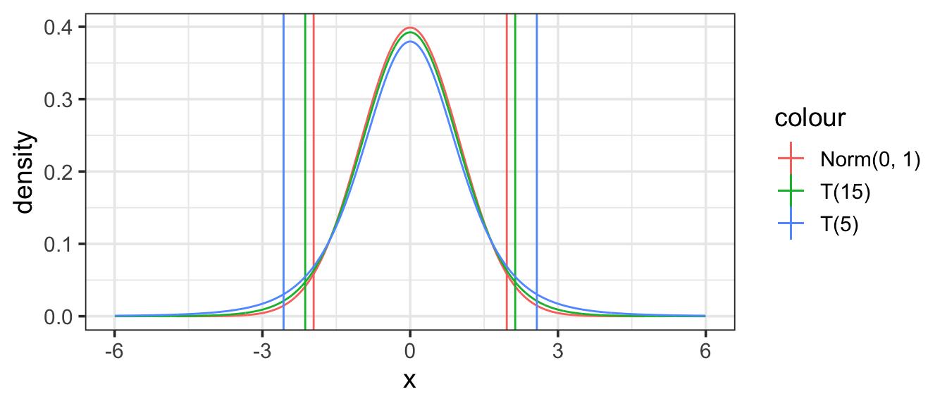
The distribution used to determine what number to use as our multiplier is calle the Student’s t-distribution. Compared to a standard normal distribution, a t-distribution will be a bit shorter and more spread out – so we have to go farther from the center to capture the middle 95% of the distribution.
To summarize, our confidence intervals will have the form
\[ \mathrm{estimate} \pm t_* SE \]
where \(t_*\) is the appropriate percentile of a t-distribution with \(n-p\) degrees of freedom. For a 95% confidence interval, we need the 2.5-percentile and the 97.5-percentile (so 95% of the t-distribution is between the two percentiles).
In addition to the decreased precision, there are other problems with using too small a data set. In particular, it is much harder to diagnose whether the model is working well or poorly – whether the model should be trusted. A good rule of them is to have at least 10–15 observations for each parameter in the model. This means we need to balance the complexity of our models against the amount of data available. We can only reliably fit very simple models to small data sets.
12.3 Confidence in Predictions
When a model value is used for making a prediction, the coefficients themselves aren’t of direct interest; it’s the prediction that counts. Nevertheless, uncertainty about the values of the parameters leads to uncertainty in the predictions. The more uncertain the parameters, the more uncertain the predictions will be.
Just as the precision of each coefficient can be established, each prediction has a precision that can be described using a confidence interval.
12.3.1 Two types of predictions
There are two ways to think about the predictions made by a linear model.
The model value is an estimate of the average response over all individuals with a given set of predictor values.
The model vlue is also an estimate of the individual resopnse for a particular individual with a given set of predictor values.
The first of these can be estimated more precisely than the second. This is because the second involves some additional variability: the variability from individual to individual. There is uncertainty both in our estimate of the average response and in how far an individual might be above or below that average.
Example 12.3 (How tall will Bill be?) To illustrate, consider making a prediction of a child’s adult height when you know the heights of the mother and father and the child’s sex. Using Galton’s data from the 19th century, a simple and appropriate model is height ~ sex + mother + father.
| term | estimate | std.error | statistic | p.value |
|---|---|---|---|---|
| (Intercept) | 15.3448 | 2.7470 | 5.59 | 0.0000 |
| sexM | 5.2260 | 0.1440 | 36.29 | 0.0000 |
| mother | 0.3215 | 0.0313 | 10.28 | 0.0000 |
| father | 0.4060 | 0.0292 | 13.90 | 0.0000 |
Now consider a hypothetical man – call him Bill – whose mother is 67 inches tall and whose father is 69 inches tall. According to the model formula, Bill’s predicted height is
\[ 15.3448 + 5.226 + 0.3215 \cdot 67 + 0.406 \cdot 69 = 70.13 \ \mathrm{inches} \]
But how precise is this prediction? One way to calculate a confidence interval on a model value is similar to bootstrapping for a coefficient.
Create many resampled data sets.
For each resampled data set, fit the model and calculate the model value from the resulting coefficients.
Calculate the standard error and confidence interval from the distribution of model values computed from the resampled data sets.
For Bill, the 95% confidence interval on his model height works out to be \(70.13 \pm 0.27\) inches: a precision of about a quarter of an inch. This high precision reflects the small standard errors of the coefficients which arise in turn from the large amount of data used to fit the model.
But this is a prediction of type 1 above – it does not take into account the variability from person to person (even among people whose parents had the same height). In other words, the model-value confidence interval is not so much about the uncertainty in Bill’s height as in what the model has to say about the average height for men like Bill (ie, men whose parents are the same heights as Bill’s parents).
If you are interested in what the model has to say about the uncertainty in the prediction of Bill’s height, you need to ask a different question and compute a different interval. The prediction confidence interval (or prediction interval for short) takes into account the spread of the cases around their model values: the residuals. For the model given above, the standard deviation of the residuals is 2.15 inches – a typical person varies from the model value by roughly that amount. This variability is in addition to our uncertainty in estimating the average height for men like Bill.
The prediction confidence interval must take into account both sources of uncertainty:
uncertainty in the coeffcient estimates leads to undercertainty in the model value estimate;
person to person variation in the population – even for people who share the same predictor values.
For men like Bill, the 95% prediction interval is \(70.13 \pm 4.24\) inches. This is much larger than the interval on the model values, and reflects mainly the size of the residual of actual cases around their model values. There is quite a bit of variety in the heights of men – even when their parents are the same height.
Note
The margin of error for a prediction interval does not decrease with sample size in the same was as it does for our other confidence intervals. No amount of data changes the amount of case-to-case variation in the population. We may be able to estimate it better, be we can’t reduce it. This puts a limit on the margin of prediction intervals, even if we have a large data set.
Furthermore, the prediction interval is very tightly connected to the assumption that the population is normal for each combination of the predictor variables. If there are clear signs that this is not the case, the prediction interval may not be very accurate.
Example 12.4 (Catastrophe in Grand Forks) In April 1997, there was massive flooding on the Red River in Minnesota and North Dakota, states in the northern US, due to record setting winter snows. The towns of Grand Forks and East Grand Forks were endangered and the story was in the news. I remember hearing a news report saying that the dikes in Grand Forks could protect against a flood level of 50 feet and that the National Weather Service predictions were for the river to reach a maximum of 47.5 to 49 feet. To the reporter and the city planners, this was good news. The city had never been better prepared and the preparations were paying off. To me, even knowing nothing about the area, the report was a sign of trouble. What kind of confidence interval was this 47.5 to 49? No confidence level was reported. Was it at a 50% level, was it at a 95% level? Was it a confidence interval on the model values alone or did it include the residuals from the model values? Did it take into account the extrapolation involved in handling record-setting conditions? Nothing in the news stories gave any insight into how precise previous predictions had been.
In the event, the floods reached 54.11 feet in Grand Forks, overtopping the dikes and inundating both towns. Damage was estimated to be more than $1 billion, a huge amount given the small population of the area. In the aftermath of the flood, the mayor of East Grand Forks said, understandably, “They [the National Weather Service] missed it, and they not only missed it, they blew it big.” The Grand Forks city engineer lamented, “with proper advance notice we could have protected the city to almost any elevation . . . if we had known, I’m sure that we could have protected a majority of the city.”
But all the necessary information was available at the time. The forecast would have been accurate if a proper prediction confidence interval had been given. It turns out that the quoted 47.5 to 49 foot interval was not a confidence interval at all – it was the range of predictions from a model under two different scenarios, with and without ongoing precipitation.
Looking back on the history of predictions from the National Weather Service, the typical residual was about 11% of the prediction. Thus, a reasonable 95% confidence interval might have been \(\pm 22%\), or, translated to feet, \(48 \pm 10\) feet. Had this interval been presented, the towns might have been better prepared for the actual level of 54.11 feet, well within the confidence band.
Whether a 95% confidence level is appropriate for disaster planning is an open question and reflects the balance between the costs of preparation and the potential damage. If you plan using a 95% level, the upper boundary of the interval will be exceeded something like 2.5% of the time. This might be acceptable, or it might not be.
What shouldn’t be controversial is that intervals need to come with a clear statement of what they mean. For disaster planning, a model-value confidence interval is not so useful – it’s about the quality of the model rather than the uncertainty in the actual outcome. And plans need to be made to handle the extreme weather events, not just the average weather events.
Note: Much of this example is drawn from the account by Roger Pielke (Jr. 1999).
12.4 A Formula for the Standard Error
When you do lots of simulations, you start to see patterns. Sometimes these patterns are strong enough that you can anticipate the result of a simulation without doing it. For example, suppose you generate two random vectors A and B and calculate their correlation coefficient: the cosine of the angle between them. You will see some consistent patterns. The distribution of correlation coefficients will have zero mean and it will have standard deviation of \(1/\sqrt{n}\).
Traditionally, statisticians have looked for such patterns in order save computational work. Why do a simulation, repeating something over and over again, if you can anticipate the result with a formula?
Such formulas exist for the standard error of a model coefficient. They are implemented in statistical software and used to generate the regression report. Here is a formula for computing the standard error of the coefficient on a model vector B in a model with more than one explanatory vector, e.g., A ~ B + C + D. You don’t need to use this formula to calculate standard errors; the software will do that. The point of giving the formula is to show how the standard error depends on features of the model, so that you can strategize about how to design your models to give suitable standard errors.
\[ \begin{aligned} \mbox{standard error of B coef.} &= \sqrt{SSR} \frac{1}{\sqrt{SS(B)}}\ \frac{1}{\sin( \theta )}\ \frac{1}{\sqrt{n}}\ \sqrt{\frac{n}{n-m}} \end{aligned} \]
There are five components to this formula, each of which says something about the standard error of a coefficient:
\(\sqrt{SSR}\) – The standard error is directly proportional to the size of the residuals. Larger residuals means larger standard error.
\(1/\sqrt{SS(B)}\) – This term can be made smaller
- by including more data (so there are more terms in the SS sum), and (b) by having the values of B more spread out (remember, \(SS(B)\) is related to the variance of \(B\)). This term also adjusts for the units of \(B\).
- by including more data (so there are more terms in the SS sum), and (b) by having the values of B more spread out (remember, \(SS(B)\) is related to the variance of \(B\)). This term also adjusts for the units of \(B\).
\(1/\sin(\theta)\) – This is the magnifying effect of collinearity. \(\theta\) is the angle between explanatory vector B the vector that would be found by fitting B to all the other explanatory vectors. When \(\theta\) is 90°, then \(\sin(\theta)=1\) and there is no collinearity and no magnification. When \(\theta = 45°\), the magnification is only 1.4. But for strong collinearity, the magnification can be very large: when \(\theta = 10°\), the magnification is 5.8. When \(\theta = 1°\), magnification is 57. For \(\theta = 0\), the alignment becomes a matter of redundancy, since B can be exactly modeled by the other explanatory variables. Magnification would be infinite, but statistical software will identify the redundancy and eliminate it.
\(1/\sqrt{n}\) – This reflects the amount of data. Larger samples give more precise estimates of coefficients, that is, a smaller standard error. Because of the square-root relationship, quadrupling the size of the sample will halve the size of the standard error. To improve the standard error by ten-fold requires a 100-fold increase in the size of the sample.
\(\sqrt{n/(n-m)}\) – The fitting process chooses coefficients that make the residuals as small as possible consistent with the data. This tends to underestimate the size of residuals – for any other estimate of the coefficients, even one well within the confidence interval, the residuals would be larger. This correction factor balances this bias out. \(n\) is, as always, the number of cases in the sample and \(m\) is the number of model vectors. So long as \(m\) is much less than \(n\), which it usually will be if you are following good statistical practice, the bias correction factor will be close to 1.
The formula suggests some ways to build models that will have coefficients with small standard errors.
Use lots of data: large \(n\).
Include model terms that will account for lots of variation in the response variable and thereby produce small residuals.
But avoid collinearity.
Again, we won’t need to use a formula like the one above. These formulas have been programmed into statistical software for us. But inspecting the formula can help us design better studies and understand how our linear models work.
The next section emphasizes the problems that can be introduced by collinearity.
12.5 Confidence and Collinearity
One of the key decisions that a modeler makes is whether to include an explanatory term; it might be a main term or it might be an interaction term or a transformation term.
The starting point for most people new to statistics might be summarized as follows:
- Methodologically Ignorant Approach. Include just one explanatory variable.
Most people who work with data can understand tabulations of group means (in modeling language, Y ~ 1 + G, where G is a categorical variable) or simple straight-line models (Y ~ 1 + X, where X is a quantitative variable.)
But it isn’t really much harder to include more in our models. At this point, the reader of this book should already understand how to include in a model multiple explanatory variables and interactions between them. When people first learn this, they typically start putting in lots of terms:
- Greedy Approach. Include everything, just in case.
The idea here is that you don’t want to miss any detail; the fitting technology will untangle everything.
Perhaps the word “greedy” is already signalling the problem in a metaphorical way. The poet Horace (65-8 BC) wrote, “He who is greedy is always in want.” Or Seneca (1st century AD), “To greed, all nature is insufficient.”
The flaw with the greedy approach to statistical modeling is not a moral fault. If adding a term improves your model, go for it! The problem is that, sometimes, adding a term can hurt the model by dramatically inflating standard errors.
To illustrate, consider a set of models of wage from the Current Population Survey 85 dataset: CPS85. A relatively simple model might take just the worker’s education into account: wage ~ 1 + educ:
| term | estimate | std.error | statistic | p.value |
|---|---|---|---|---|
| (Intercept) | -0.746 | 1.045 | -0.714 | 0.4758 |
| educ | 0.750 | 0.079 | 9.532 | 0.0000 |
The coefficient on educ says that a one-year increase in education is associated with a wage that is higher by 75 cents/hour. (Remember, these data are from the mid-1980s.) The standard error is 8 cents/hour per year of education, so the confidence interval is \(75 \pm 16\) cents/hour per year of education.
A slightly more elaborate model includes age as a covariate. This might be important because education levels typically are lower in older workers, so a comparison of workers with the same level of education ought to hold age constant. A simple adjustment will take that into account. Here’s the regression table on the model wage ~ 1 + educ + age:
| term | estimate | std.error | statistic | p.value |
|---|---|---|---|---|
| (Intercept) | -5.534 | 1.279 | -4.326 | 0.00002 |
| educ | 0.821 | 0.077 | 10.657 | 0.00000 |
| age | 0.105 | 0.017 | 6.112 | 0.00000 |
In this new model, the coefficient on educ changed slightly from 75 to 82 cents/hour per year of education while leaving the standard error more or less the same.
Of course, wages also depend on experience. Every year of additional education tends to cut out a year of experience. Here is the regression report from the model wage ~ 1 + educ + age + exper:
| term | estimate | std.error | statistic | p.value |
|---|---|---|---|---|
| (Intercept) | -4.770 | 7.043 | -0.68 | 0.4985 |
| educ | 0.948 | 1.155 | 0.82 | 0.4121 |
| age | -0.022 | 1.155 | -0.02 | 0.9845 |
| exper | 0.128 | 1.156 | 0.11 | 0.9122 |
Look at the regression table carefully. The standard errors have exploded! The confidence interval on educ is now \(95 \pm 231\) cents/hour per year of education – a very imprecise estimate. Indeed, the confidence interval now includes zero, so the model is consistent with the skeptic’s claim that education has no effect on wages, once you hold constant the level of experience and age of the worker.
A better interpretation is that greed has gotten the better of the modeler. The large standard errors in this model reflect a deficiency in the data: the multi-collinearity of exper with age and educ as described in in the example in Section 8.4.
A simple statement of the situation is this:
Collinearity and multi-collinearity cause model coefficients to become less precise – they increase standard errors.
This doesn’t mean that you should never include model terms that are collinear or multi-collinear. If the precision of your estimates is good enough, even with the collinear terms, then there is no problem. You, the modeler, can judge if the precision is adequate for your purposes.
The estimate \(95 \pm 231\) cents/hour is probably not precise enough for any reasonable purpose. Including the exper term in the model has made the entire model useless, not just the exper term, but the other terms as well! That’s what happens when you are greedy.
The good news is that you don’t need to be afraid of trying a model term. Use the standard errors to help judge when your model is acceptable and when you need to think about dropping terms due to collinearity.
12.5.1 Aside: Redundancy and Multi-collinearity
Redundancy can be seen as an extreme case of multi-collinearity. So extreme that it renders the coefficients completely meaningless. That’s why statistical software is written to delete redundant vectors. With multi-collinearity, things are more of a judgment call. The judgment needs to reside in you, the modeler.
12.6 Confidence and Bias
The margin of error tells you about the precision of a coefficient: how much variation is to be anticipated due to the random nature of sampling. It does not, unfortunately, tell you about the accuracy of the coefficient; how close it is to the “true” or “population” value.
A coefficient makes sense only within the context of a model. Suppose you fit a model Y ~ A + B. Then you think better of things and look at the model Y ~ A + B + C. Unless variable C happens to be orthogonal to A and B, the coefficients on A and B are going to change from the first model to the second.
If you take the point of view that the second model is “correct,” then the coefficients you get from the first model are wrong. That is, the omission of D in the first model has biased the estimates of A and B.
On the other hand, if you think that the model Y ~ A + B reflects the “truth,” then the coefficients on A and B from Y ~ A + B + C are biased.
The margin of error from any model tells you nothing about the potential bias. How could it? In order to measure the bias you would have to know the “correct” or “true” model.
The issue of bias often comes down to which is the correct set of model terms to include. This is not a statistical issue – it depends on how well your model corresponds to reality. Since people disagree about reality, perhaps it would be best to think about bias with respect to a given theory of how the world works. A model that produces unbiased coefficients according to your theory of reality might give biased coefficients with respect to someone else’s theory. Avoiding bias is a difficult matter and it’s hard to know when you have succeeded. A very powerful but challenging strategy is to intervene to make your system simpler, so that every modeler’s theories can agree. See Chapter 18.
12.7 Checking Regression Assumptions
12.7.1 What are the regression assumptions?
The linear model formula looks like this:
\[ Y = \underbrace{\beta_0 + \beta_1 x_1 + \beta_2 x_2 + \cdots \beta_k n_k}_{\mbox{linear part}} + \underbrace{\varepsilon}_{\mbox{error}} \]
This describes a relationship for the entire population. We don’t expect that response values (\(Y\)) to be exactly what the linear model specifies – even for the correct values of the \(\beta\)’s. \(\varepsilon\) (“epsilon”) measures the difference between the two and is called the “error”.
We don’t know the best values for the \(\beta\)’s (the ones that fit best for the entire population), but we can estimate them from our sample.
That’s called fitting the model.
For each row in our data, we get this relationship:
\[ Y = \underbrace{\hat \beta_0 + \hat \beta_1 x_1 + \hat \beta_2 x_2 + \cdots \hat \beta_k n_k}_{\mbox{linear part}} + \underbrace{e}_{\mbox{residual}} \]
The formulas used to calculate the standard errors (and intervals) we have been using all suppose certain things these formulas. As we will see, we can investigate the residuals to see how plausible the suppositions are.
Here are four assumptions that conviently spell out LINE:
Linear relationship
The relationship between response and predictors is the one described by our linear model. That is, we have the correct model formula.
For a simple linear model (just one quantitative predictor and an intercept), we can assess this by looking at a scatter plot. For more complicated models we learn other ways to investigate. But either way the caution is:
Don’t fit a line (linear model) if a line (linear model) doesn’t fit.
The computer is happy to fit any model to any data, even if it is a bad idea.
Independent errors
The response values don’t all match the model values exactly. But the differences between the model values and the response values should be independent. The is the large and small errors should not cluster in any systematic way, it should just be random where the large and small errors occur.
Normal errors
Furthermore, the shape of the distribution of these errors should be a normal distribution (centered at 0).
Equal variance
The standard deviation of that normal distribution can be anything, but it should be the same everywhere. (The fancy term for this is the tongue-twisting homoskedasticity; the opposite is the equally tongue-twisting hetreoskedasticity.)
This call be succinctly written as
\[ Y = \underbrace{\beta_0 + \beta_1 x_1 + \beta_2 x_2 + \cdots \beta_k n_k}_{\mbox{linear part}} + \underbrace{\varepsilon}_{\mbox{error}} \quad \mbox{and} \quad \varepsilon \stackrel{ind}{\sim} \mathsf{Norm}(0, \sigma) \] These assumptions are all about the error term \(\varepsilon\). And our best way to understand what the error terms might be in the population is to look at the residuals in our data.
Investigating residuals is the key to checking the model assumptions.
12.7.2 Distribution of Residuals
We can check the overall distribution of residuals using a histogram or density plot. For example, here are plots showing the distribution of the residuals for the model net ~ age + sex using our random sample of 50 runners:
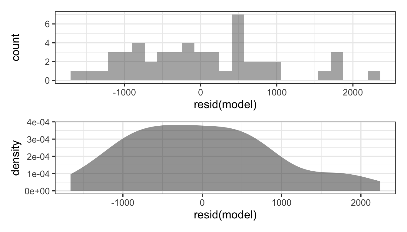
We would like to see that this distribution is unimodal (one major peak) and roughly symmetric (not clearly skewed on direction or the other). The larger the data set, the less this matters. Unfortunately, when it matters most (small data sets) it is also hardest to judge – shape is hard to judge from only a few values.
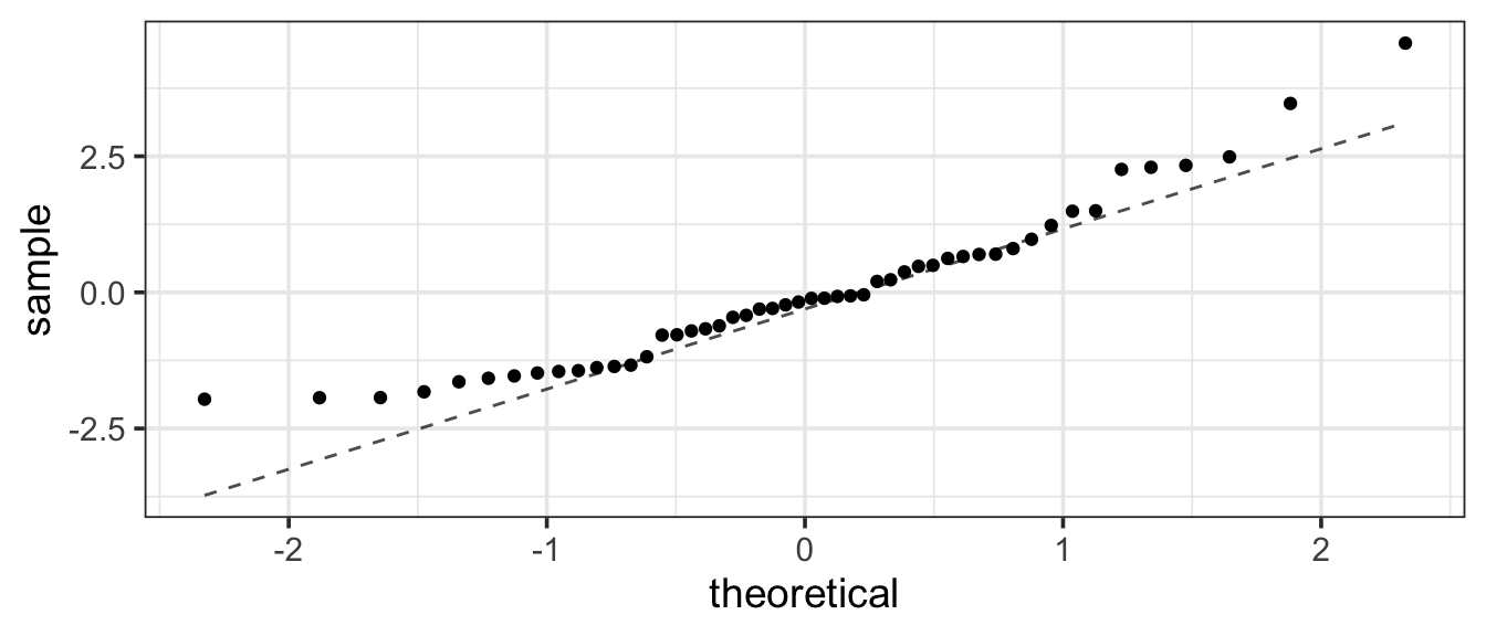
Since our eyes are not particularly good at judging curvey shapes, there is another plot called a normal-quantile plot that has been designed so that for perfectly normal data, the shape will be a line. Actual data will always have a bit of jaggediness too it, so we are looking to see if the overall impression is of something other than a line.

That looks pretty good. The few smallest residuals are not quite as negative as the largest ones are positive, so there seems to be some mild skew.
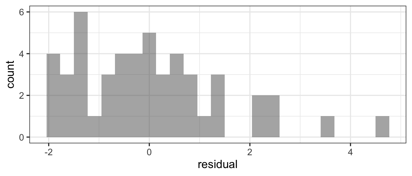
Here’s an example that doesn’t look quite as good:
In Figure 12.5, the curved pattern is more pronounced. The most negative residuals should be more negative and the most positive ones less positive if this were a normal distribution. This indicates a skewed (right) distribution. Residuals always have a mean of 0. Notice how the range is from about -2 to 4 – the large residuals stretch twice as far above the mean as the small ones are below the mean. We can see this in a histogram as well.
Note
The linear regression framework does not specify any particular distribution of the predictors or of the response, only for the difference between response values and modeled resonse values (the errors or residuals). So don’t worry if those other things have distributions that are not normal.
12.7.3 Residuals vs Fits
Another useful plot is a residuals vs fits plot

net ~ age + sex.Here we are hoping to see a random jumble of points. Any systematic patterns here could indicate problems. This plot looks pretty good.
Here are three examples of things that don’t look so good.
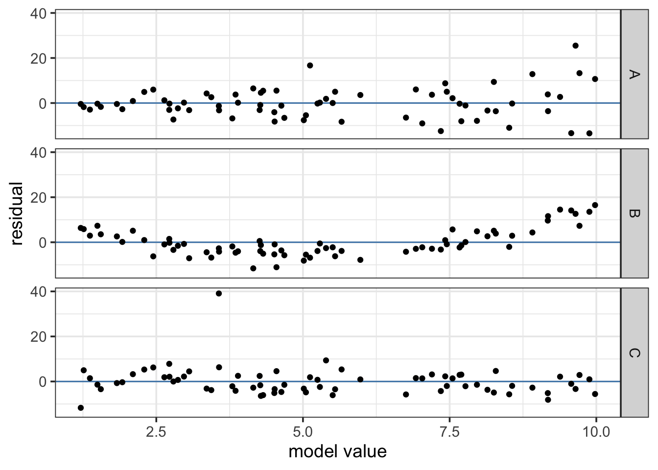
In example A, the residuals seem to be getting larger as we move from left to right.
It seems that when our model makes larger predictions, those predicts are also less precise. But the regression framework assumes the predictions are equally precise everywhere.
In example B, there is a clear curve.
The residuals on the ends are positive and in the middle tend to be negative. This is an indication that we may not have a linear relationship between the reponse and the predictors – at least not the one specified by the model.
In example C, there is one residual that seems much larger than the rest.
Unfortunately, linear models can be quite sensitive to a few values that stick out like this – especially if they are near the extremes of the data. We might try fitting our model with and without these cases. If things don’t change much, then we don’t have to worry to much. If things do change a lot, then these unusual values are having an outsized impact on the model. There are formal ways to quantify this affect. But even without formal methods, it is good to be aware of this potential problem.
12.7.4 Residuals vs other things
We can also make scatter plots showing residuals vs other things like
time
The residuals should not show any tendencies related to time. If they do, we may need to do time series analysis or at least include time in our model.
order of observations in the data
This might be a proxy for time or it might be a proxy for something else. Again, we don’t want to see patterns here.
a variable not in the model
If there appears to be a strong relationship between our residuals (the unexplained variation) and some unused variable, that is an indication that the unused variable provides an explanation for what is unexplained in our model. So perhaps we should include it in the model! That’s exactly how we improve our models – by including something that explains what the current model cannot.
12.7.5 Why not residuals vs a predictor already in the model?
You may wonder why residuals vs a predictor was not in the previous list.
Two reasons:
In the case of a simple linear model (one quantitative predictor and an intercept), a plot of residuals vs fits reveals exactly the same information as a plot of residuals vs the predictor. So it would be OK to do residuals vs predictor here (and perhaps easier to explain to your colleagues). But it doesn’t reveal any new information.
For a model with multiple predictors, the model assumptions are not about the relationship between each predictor and the response but betwen the full model values – those fitted values – and the observed reponses. So checking against one predictor isn’t really checking the right thing.
So best to get used to thinking about residuals vs model values (fitted values).
12.7.6 The size of residuals
Note: the model assumptions don’t say anything about how large or small residuals should be. They just need to be normal, independent, and have the same variance. If they are larger, it just means \(\sigma\) is larger, but the model is fine with that.
Of course, smaller residuals means we are doing a better job of explaining what’s going on and can make better predictions. But that is a different issue.
Larger residuals just means that our estimates are not very precise, but that will be accurately quantified by our confidence intervals.
Violating the other assumptions means that our confidence intervals may be wrong, so they won’t accurately reflect the precision in the first place. That’s a more serious problem.
12.8 What to do if there are problems
Having a way to find problems isn’t very comforting if there is nothing to be done about it. Fortunately, thre are often things we can do, like
Use a different model.
Using different predictors, or adding an interaction or transformation term might make all the difference.
Use a different method.
We won’t talk much about other methods in this class, but we don’t have to assume that the error terms are normal. We could specify some other distribution. But that requires additional analysis methods – generalized linear models, for example – that we won’t see in this course.
Use resampling.
Resampling doesn’t specify any particular distribution for the error terms, which seems ideal. But it only works well if the sample provides a good representation of whatever that distribution happens to be. Futhermore, it is slower, and not all statistical software supports it well. Nevertheless, you will see resampling methods more and more often since modern computers have made these methods feasible.