11 Modeling Randomness
The race is not to the swift, nor the battle to the strong, neither yet bread to the wise, nor yet riches to men of understanding, nor yet favor to men of skill; but time and chance happeneth to them all. – Ecclesiastes
Until now, emphasis has been on the deterministic description of variation: how explanatory variables can account for the variation in the response. Little attention has been paid to the residual other than to minimize it in the fitting process.
It’s time now to take the residual more seriously. It has its own story to tell. By listening carefully, the modeler gains insight into even the deterministic part of the model. Keep in mind the definition of statistics offered in Chapter 1:
Statistics is the explanation of variability in the context of what remains unexplained.
The next two chapters develop concepts and techniques for dealing with “what remains unexplained.” In later chapters these concepts will be used when interpreting the deterministic part of models.
11.1 Describing Randomness
Consider a process whose outcome is completely random, for instance, the process of flipping a coin. How do we describe and study such random processes? We do this by answering two questions:
What are the possible results of the random process?
How likely are the various results to occur?
11.1.1 Outcome Set
The outcome set or set of outcomes1 of a random process tells us what could result from the random process. With a coin, for instance, the outcome must be “heads” or “tails” – it can’t be “rain.” So the outcome set contains just “heads” and “tails” (which we might abbreviation as H and T). This answers the first question for the toss of a fair coin.
11.1.2 Probability
A probability model assigns a probability to each event.
An event is just a set of some of the outcomes. (Note: mathematicians consider “none” and “all” to be “some”.) A probability is a number between 0 and 1. A probability of 0 means “impossible.” A probability of 1 means “certain.” Probabilities closer to 1 indicate that an event is more likely than probabilities closer to 0.
For the flip of a fair coin, one imagines that the two outcomes are equally likely, so they should have equal probabilities. These probabilities should sum to 1 (since they are the only possible outcomes). So for a fair coin, a good probability model specifies that the probability of heads is 1/2 and the probability of tails is 1/2.
When the number of outcomes in the outcome set is small, we can represent a probability model with a probability table. The probability table for the fair coin model looks like this
Probability table for a fair coin
| outcome | heads | tails |
|---|---|---|
| probability | 1/2 | 1/2 |
What makes a coin flip random is not that the probability model assigns equal probabilities to each outcome. If coins worked differently, an appropriate probability model might be
Probability table for an “unfair” coin
| outcome | heads | tails |
|---|---|---|
| probability | 0.6 | 0.4 |
The reason the flip is (purely) random is that the probability model contains all the information; there are no explanatory variables that account for the outcomes in any way.
Example 11.1 (Rolling a Die) The outcome set is \(\{1, 2, 3, 4, 5, 6\}\) – the six possible numbers that could appear on the die. If the die is a fair die, each of these outcomes will be equally likely, so the probability model assigns probability 1/6 to each of the outcomes.
Probability table for a fair die
| Outcome | 1 | 2 | 3 | 4 | 5 | 6 |
|---|---|---|---|---|---|---|
| Probability | 1/6 | 1/6 | 1/6 | 1/6 | 1/6 | 1/6 |
Now suppose that the die is “loaded.” This is done by drilling into the dots to place weights in them. In such a situation, the heavier sides are more likely to face down. Since 6 is the heaviest side, the most likely outcome would be a 1. (Opposite sides of a die are arranged to add to seven, so 1 is opposite 6, 2 opposite 5, and 3 opposite 4.) Similarly, 5 is considerably heavier than 2, so a 2 is more likely than a 5. An appropriate probability model is this:
Probability table for a loaded die
| Outcome | 1 | 2 | 3 | 4 | 5 | 6 |
|---|---|---|---|---|---|---|
| Probability | 0.28 | 0.22 | 0.18 | 0.16 | 0.10 | 0.06 |
One view of probabilities is that they describe how often outcomes occur. For example, if you conduct 100 trials of a coin flip, you should expect to get something like 50 heads. According to the frequentist view of probability, you should base a probability model of a coin on the relative proportion of times that heads or tails comes up in a very large number of trials.
Another view of probabilities is that they encode the modeler’s assumptions and beliefs. This view gives everyone a license to talk about things in terms of probabilities, even those things for which there is only one possible trial, for instance current events in the world. To a subjectivist , it can be meaningful to think about current international events and conclude, “there’s a one-quarter chance that this dispute will turn into a war.” Or, “the probability that there will be an economic recession next year is only 5 percent.”
Example 11.2 (The Chance of Rain) Tomorrow’s weather forecast calls for a 10% chance of rain. Even though this forecast doesn’t tell you what the outcome will be, it’s useful; it contains information. For instance, you might use the forecast in making a decision not to cancel your picnic plans.
But what sort of probability is this 10%? The frequentist interpretation is that it refers to seeing how many days it rains out of a large number of trials of identical days. Can you create identical days? There’s only one trial – and that’s tomorrow. The subjectivist interpretation is that 10% is the forecaster’s way of giving you some information, based on his or her expertise, the data available, etc.
Saying that a probability is subjective does not mean that anything goes. Some probability models of an event are better than others. There is a reason why you look to the weather forecast on the news rather than gazing at your tea leaves. There are in fact rules for doing calculations with probabilities: a “probability calculus.”
Subjective probabilities are useful for encoding beliefs, but the probability calculus should be used to work through the consequences of these beliefs. The Bayesian philosophy of probability emphasizes the methods of probability calculus that are useful for exploring the consequences of beliefs.
Example 11.3 (Flipping two coins) You flip two coins and count how many heads you get. The outcome space is 0 heads, 1 head, and 2 heads. What should the probability model be? Here are two possible models:
Model 1
| number of heads | 0 | 1 | 2 |
|---|---|---|---|
| probability | 1/3 | 1/3 | 1/3 |
Model 2
| number of heads | 0 | 1 | 2 |
|---|---|---|---|
| probability | 1/4 | 1/2 | 1/4 |
If you are unfamiliar with probability calculations, you might decide to adopt Model 1. However heartfelt your opinion, though, Model 1 is not as good as Model 2. Why? Given the assumptions that a head and a tail are equally likely outcomes of a single coin flip, and that there is no connection between successive coin flips – that they are independent of each other – the probability calculus leads to the 1/4, 1/2, 1/4 probability model.
How can you assess whether a probability model is a good one, or which of two probability models are better? One way is to compare observations to the predictions made by the model. To illustrate, suppose you actually perform 100 trials of the coin flips in example above and you record your observations. Each of the models also gives a prediction of the expected number of outcomes of each type:
Model 1
| value | 0 | 1 | 2 |
|---|---|---|---|
| predicted count | 33.3 | 33.3 | 33.3 |
Model 2
| value | 0 | 1 | 2 |
|---|---|---|---|
| predicted count | 25 | 50 | 25 |
The discrepancy between the model predictions and the observed counts tells something about how good the model is. A strict analogy to linear modeling would suggest looking at the residual: the difference between the model values and the observed values. For example, you might look at the familiar sum of squares of the residuals. For Model 2 this is
\[ (28-25)^2 + (45-50)^2 + (27-25)^2 \]
More than 100-years ago, it was worked out that for probability models this is not the most informative way to calculate the size of the residuals. It’s better to adjust each of the terms by the model value, that is, to calculate
\[ (28-25)^2/25 + (45-50)^2/50 + (27-25)^2/25 \]
The details of the measure are not important right now, just that there is a way to quantify how well a probability model matches the observations.
11.2 Families of Probability Models
It turns out that there is a reasonably small set of standard probability models that apply to a wide range of settings. You don’t always need to derive probability models, you can use the ones that have already been derived. This simplifies things dramatically, since you can accomplish a lot merely by learning which of the familiar models might apply in a given setting.
These probability models come in families of related models. For example, a fair coin and an unfair coin come from the same family. In each case there are two possible outcomes (heads and tails). What differs is the probability of getting heads, \(p\). This number \(p\) distinguishes one member of the family from another. A number like this that distinguishes members of a family of probabilty models is called a parameter.
Each of the probability models we will introduce has one or more parameters. These parameters can be used to adjust the models to the particular details of a setting. In this sense, the parameters are akin to the model coefficients that are set when fitting models to data.
The rest of this chapter will introduce several commonly occuring families of probability models.
11.3 Models of Counts
11.3.1 The Binomial Model
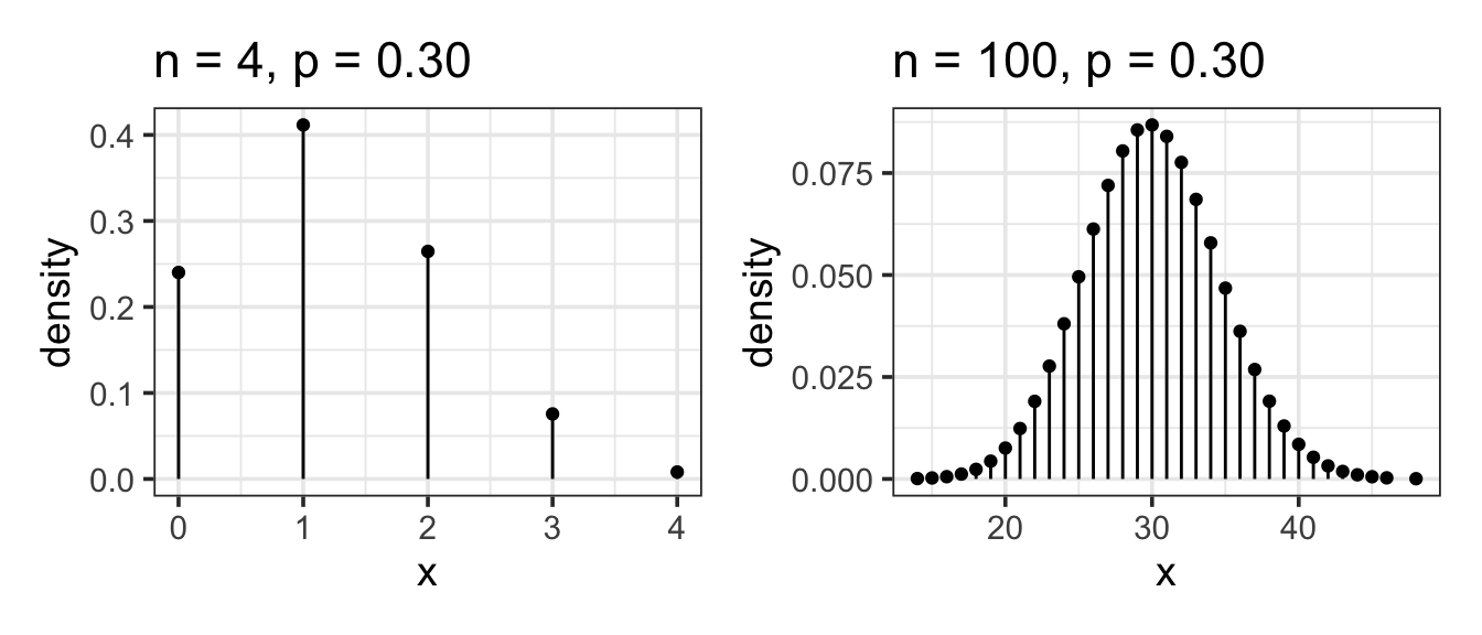
Definition 11.1 (Binomial Model) Setting. The standard example of a binomial model is a series of coin flips. A coin is flipped n times and the outcome of the event is a count: how many heads. The outcome space is the set of counts 0, 1, …, n.
To put this in more general terms, the setting for the binomial model is an event that consists of n trials. Each of those trials is itself a purely random event where the outcome set has two possible values. For a coin flip, these would be heads or tails. For a medical diagnosis, the outcomes might be “cancer” or “not cancer.” For a political poll, the outcomes might be “support” or “don’t support.” All of the individual trials are identical and independent of the others.
The name binomial – “bi” as in two, “nom” as in name – reflects these two possible outcomes. Generically, they can be called “success” and “failure.” The outcome of the overall event is a count of the number of successes out of the n trials.
Parameters. The binomial model has two parameters: the number of trials n and the probability p of success in each trial.
Example 11.4 (Multiple Coin Flips) Flip 10 coins and count the number of heads. The number of trials is 10 and the probability of “success” is 0.5. Here is the probability model:
Example 11.5 (Houses for Sale) Count the number of houses on your street with a for-sale sign. Here n is the number of houses on your street. p is the probability that any randomly selected house is for sale. Unlike a coin flip, you likely don’t know p from first principles. Still, the count is appropriately modeled by the binomial model. But until you know p, or assume a value for it, you can’t calculate the probabilities.
11.3.2 The Poisson Model
Definition 11.2 (Poisson Model) Setting. Like the binomial, the Poisson model also involves a count. It applies when the things you are counting happen at a typical average rate. For example, suppose you are counting cars on a busy street on which the city government claims the typical traffic level is 1000 cars per hour. You count cars for 15 minutes to check whether the city’s claimed rate is right. According to the rate, you expect to see 250 cars in the 15 minutes. But the actual number that pass by is random and will likely be somewhat different from 250. The Poisson model assigns a probability to each possible count.
Parameters. The Poisson model has only one parameter: the average rate at which the events occur. Often the rate is denoted with the Greek letter \(\lambda\) (lambda).
Example 11.6 (The Rate of Highway Accidents) In your state last year there were 300 fatal highway accidents: a rate of 300 per year. If this rate continued, how many accidents will there be today?
Since you are interested in a period of one day, divide the annual rate by 365 to give a rate of 300/365 = 0.8219 accidents per day. According to the Poisson model, the probabilities are:
| Outcome | 0 | 1 | 2 | 3 | 4 | 5 |
|---|---|---|---|---|---|---|
| Probability | 0.440 | 0.361 | 0.148 | 0.041 | 0.008 | 0.001 |
People often confuse the binomial setting with the Poisson setting. Notice that in a Poisson setting, there is not a fixed number of trials, just a typical rate at which events occur. The count of events has no firm upper limit. In contrast, in a binomial setting, the count can never be higher than the number of trials, n.

11.4 Quantiles (Percentiles, Deciles, Quartiles, etc.)
Percentiles. Students who take standardized tests know that the test score can be converted to a percentile: the fraction of test takers who got that score or less. Similarly, each possible outcome of a random variable falls at a certain percentile. It often makes sense to refer to the outcomes by their percentiles rather than the value itself. For example, the 90th percentile is the value of the outcome such that 90 percent of the time a random outcome will be at that value or smaller.
Deciles and quartiles are the same thing as percentiles, just expressed in tenths or quarters instead of hundredths.
The third decile is the 30th percentile – both say that 30% of the distribution are below that value.
The first quartile is the 25th percentile – both say that 25% of the distribution fall below that value.
The general term for this is a quantile, which is expressed as a fraction or decimal between 0 and 1.
- The 0.975 quantile is the value that has 97.5% of the distribution below that value.
Percentiles are used, for instance, in finding what range of outcomes is typical, as in calculating a coverage interval for the distribution.
11.4.1 Forwards and backwards
We can ask quantile questions in one of two directions:
we might know the value in the distribution and want to know what percentage of the distribution lies below that value – we want to know the percentile. This is what happens we want to know how unusual (or not) a particular value is.
we might know the percentage we would like to have below some value, but not know what that value is. Coverage intervals work this way – we specify the percentage of coverage and determine the values on either end of the interval.
Software can be used to answer both types of questions for common distributions or for data distributions.
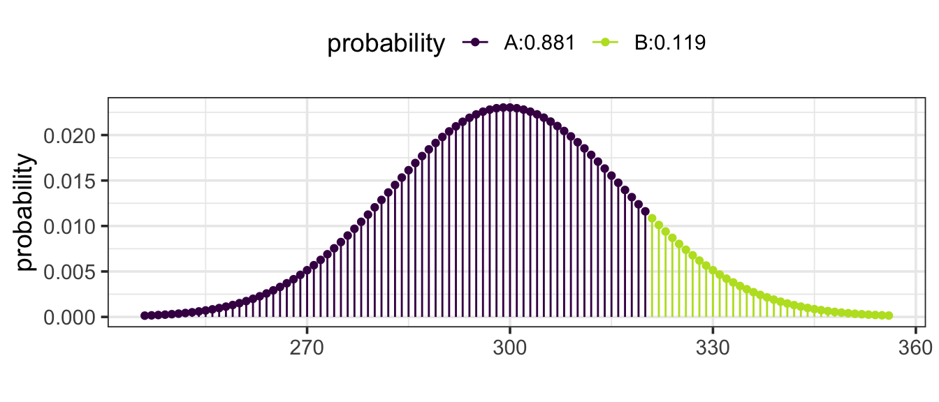
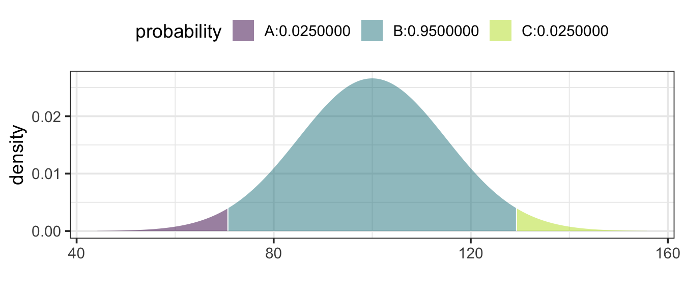
Example 11.7 (A Political Poll) You conduct 500 interviews with likely voters about their support for the incumbent candidate. You believe that 55% of voters support the incumbent. What is the likely range in the results of your survey?
This is a binomial setting, with parameters n = 500 and p = 0.55. It’s reasonable to interpret “likely range” to be a 95% coverage interval. The boundaries of this interval are the 2.5- and 97.5-percentiles (the 0.025 and 0.975 quantiles) of this binomial distribution. Software can be use to determine that these values are 253 and 297, respectively. That is 253 is the 2.5-percentile and 297 is the 97.5 percentile.
Example 11.8 (A typical year or atypical year?) Last year there were 300 highway accidents in your state. This year saw an increase to 321. Is this a likely outcome if the underlying rate hadn’t changed from 300?
This is a Poisson setting, with the rate parameter at 300 per year. According to the Poisson model, the probability of seeing 321 or more is 0.119: not so small. That is 321 is the 88.1 percentile – on the high side but not unusually so.
11.5 Models of Continuous Outcomes
The binomial and Poisson models apply to settings where the outcome is a count. There are other settings where the outcome is a number that is not necessarily a counting number but can take on any value in some range.
11.5.1 Area = Probability
Continous random variables are described by a curve. The area underneath the curve represents probability. This means that
Where the curve is higher, values are more likely.
Where the curve is lower, values are less likely.
The total area under the curve must be 1 (100%).
Such a curve is called a density curve or a density function.
For continuous random variables, it does not make sense to ask about the probability of taking on a specific value, instead, we ask about the probability of the random value being within some interval. For example, we might as about the probablity that the random value is between 5 and 10. The answer to this would be equal to the area under the density curve and between 5 and 10.

These areas are generally computed using software, but if you have taken calculus, you will know that integration is the tool that computes these probabilities because integrals can be interpreted as the area under a curve.
11.5.2 The Uniform Model
Uniform Model
Setting. A random number is generated that is equally likely to be anywhere in some range. An example is a spinner that is equally likely to come to rest at any orientation between 0 and 360 degrees.
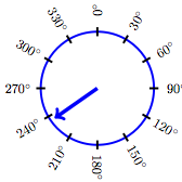
Parameters. Two parameters: the upper and the lower end of the range.

Example 11.9 (Uniform(0, 1)) A uniform random number is generated in the range 0 to 1. What is the probability that it will be smaller than 0.05?
Answer: 0.05. This area is easily computed because the shape of the density curve is so simple. It’s height must be 1 between 0 and 1 (to make the total area equal to 1.) To get the desired probability, we compute the area of the rectangle shaded below. It is 0.05 units wide and 1 unit tall, so the area is \(0.05 \cdot 1 = 0.05\).

(Simple as it seems, this particular example will be relevant in studying p-values in a later chapter.)
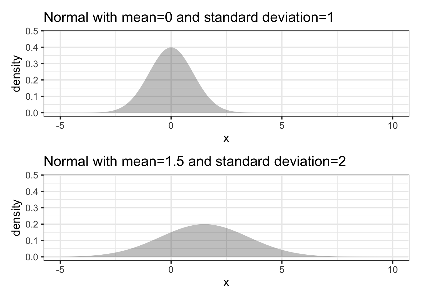
11.5.3 The Normal Model
Setting. The normal model turns out to be a good approximation for many purposes, thus the name “normal.” When the outcome is the result of adding up lots of independent numbers, the normal model often applies well. In statistical modeling, model coefficients are calculated with dot products, involving lots of addition. Thus, model coefficients are often well described by a normal model.
The normal model is so important that we will spend considerably more time with this type of distribution than with the others.
Parameters. Two. The mean which describes the most likely outcome, and the standard deviation which describes the typical spread around the mean.
Shape. Normal distributions are symmetric with a “bell shape”. If you have heard someone metion “the bell curve”, then it is probably the normal denisty curve that they were talking about. Different normal distributions might be taller and skinner or shorter and wider, but all of them have the same basic bell shape.
Example 11.10 (IQ Test Scores) Scores on a standardized IQ test are arranged to have a mean of 100 points and a standard deviation of 15 points. What’s a typical score from such a test?
Answer: According to the normal model, the 95% coverage interval is 70.6 to 129.4 points.
11.5.4 The Log-normal Model
Setting. The normal distribution is widely used as a general approximation in a large number of settings. However, the normal distribution is symmetrical and fails to give a good approximation when a distribution is strongly skewed. The log-normal distribution is often used when the skew is important. Mathematically, the log-normal model is appropriate when taking the logarithm of the outcome would produce a bell-shaped distribution.
Parameters. In the normal distribution, the two parameters are the mean and standard deviation. Similarly, in the log-normal distribution, the two parameters are the mean and standard deviation of the log of the values.
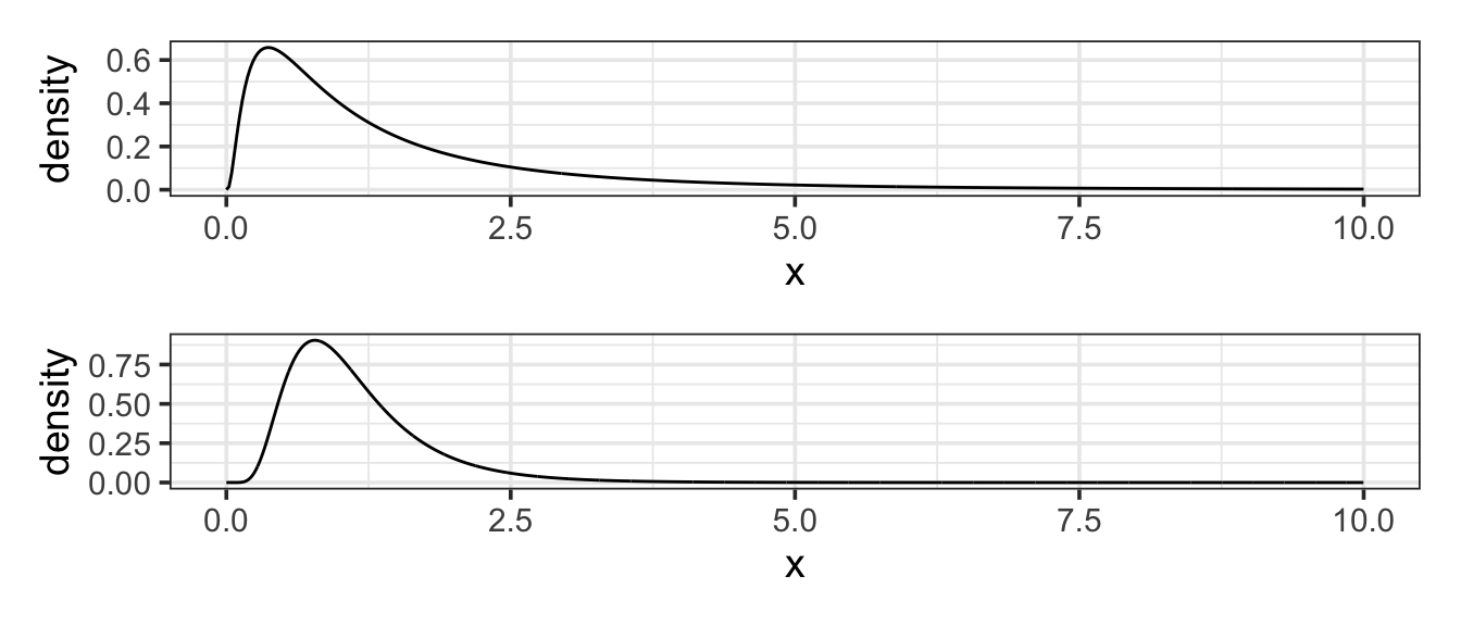
Example 11.11 (High Income) In most societies, incomes have a skewed distribution; very high incomes are more common than you might expect. In the United States, for instance, data on middle-income families in 2005 suggests a mean of about $50,000 per year and a standard deviation of about $20,000 per year (taking “middle-income” to mean the central 90% of families). If incomes were distributed in a bell-shaped, normal manner, this would imply that the 99th percentile of income would be $100,000 per year. But this understates matters. Rather than being normal, the distribution of incomes is better approximated with a log-normal distribution(Montroll and Schlesinger 1983). Using a log-normal distribution with parameters set to match the observations for middle-income families gives a 99th percentile of $143,000.
11.5.5 The Exponential Model
Setting. The exponential model is closely related to the Poisson. Both models describing a setting where events are happening at random but at a certain average rate. The Poisson describes how many events happen in a given period of time. In contrast, the exponential model describes the spacing between events.
Parameters. Just like the Poisson, the exponential model has one parameter, the rate (often denoted \(\lambda\)).
Shape. All exponential distributions have the same basic shape with a peak at 0 and falling off from there. No values can be less than 0. The rate parameter controls how quickly things fall off from 0. The lower the rate, the longer it might be until an event occurs.
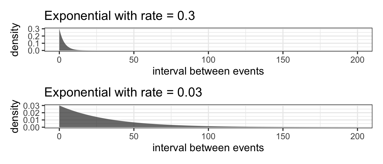
Example 11.12 (Times between Earthquakes) In the last 202 years from 1804 to 2005, there have been six large earthquakes in the Himalaya mountains, including one in 2005. [See update below.] This suggests a typical rate of 6 / 202 = 0.03 earthquakes per year – about one every 33 years. Of course, sometimes there will be more than 33 years between earthquakes, sometimes less.
If earthquakes follow the Poisson/exponential model, what is the probability that there will be another large earthquake in a 10 year interval?
We can answer this two ways.
Using an exponential model with rate 0.03 (0.03 earthquakes per year).
The probability question is the probability that the time between large earthquakes is at less than 10 years.
Using a Poisson model with rate 0.3 (0.3 earthquakes every 10 years).
Now the question becomes what is the probability of getting a count of at least 1. (This is the same as asking what is the probability that the count is not 0.)
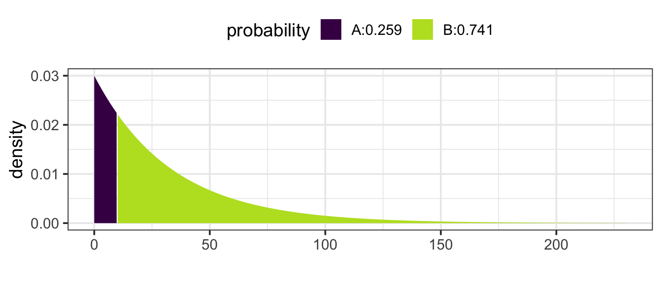
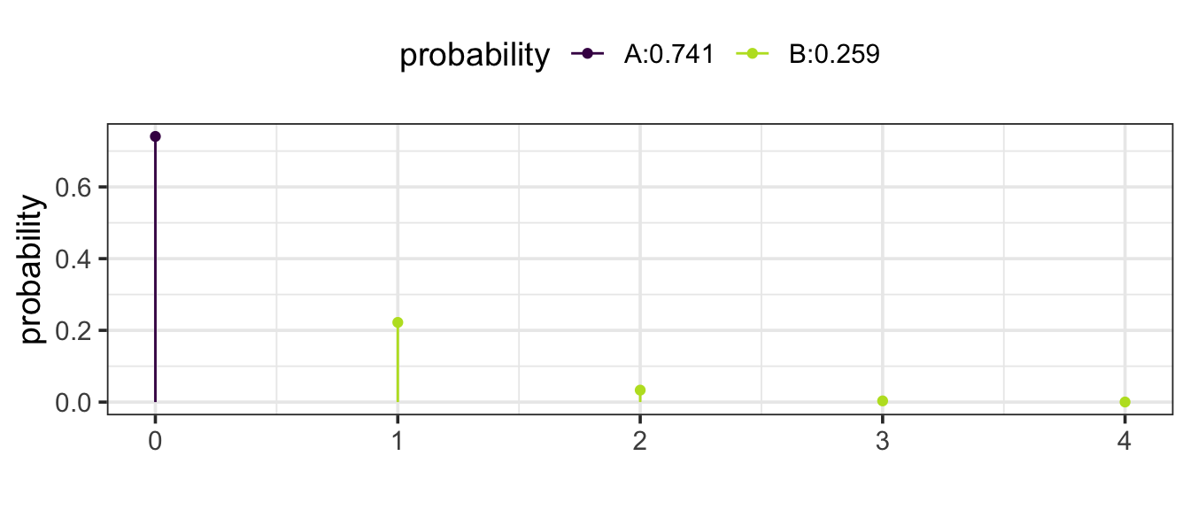
Either way we get the same answer: 0.259 or 25.9%.
You might be surprised the probability is that large. But remember that the exponential/Poisson model does not say that events occur at consistent intervals. Some gaps will be larger, some smaller. [Update: Tragically, there was another large earthquake in 2015. Events with a probability of 26% do happen.]
There can also be surprisingly large gaps between earthquakes. For instance, the probability that another large earthquake won’t occur in the next 100 years is 5% according to the exponential model.
11.6 More about Normal Distributions
The normal distributions occur so frequently that it is worth getting to know them a bit better than some of the other distributions. This is because many quantities have a roughly bell-shaped distribution so the normal model makes a good approximation in many settings.
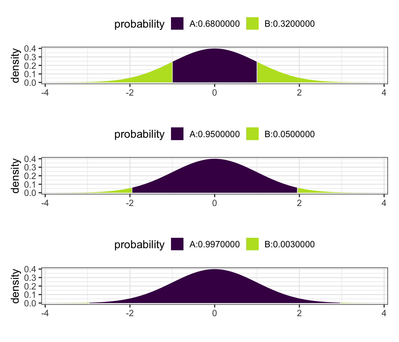
11.6.1 68-95-99.7
All normal distributions (but not other types of distributions) share an interesting property:
approximately 68% (more precisley: 68.2689492%) of the distribution is between 1 standard deviation below the mean and 1 standard deviation above the mean.
approximately 95% (more precisley: 95.4499736%) of the distribution is between 2 standard deviations below the mean and 2 standard deviations above the mean.
approximately 99.7% (more precisley: 99.7300204%) of the distribution is between 3 standard deviations below the mean and 3 standard deviations above the mean.
So these three numbers – 68, 95, 99.7 – form useful benchmarks for the normal distributions.
Because all normal distributions share this property, it is useful to think about values in a normal distribution in terms how many standard deviations above or below the mean they are. This number of standard deviations above or below the mean is called the z-score.
\[ z\mathrm{-score} = \frac{\mathrm{value} - \mathrm{mean}}{\mathrm{standard\ deviation}} \]
Example 11.13 (IQ Percentiles from Scores.) In a standard IQ test, scores are arranged to have a mean of 100 and a standard deviation of 15. A person gets an 80 on the exam. What is their z-score?
Answer: z = (80−100) / 15 = −1.33. They are 1.33 standard deviations below the mean.
Note: We know that 68% of IQ scores are between 85 and 115. Half of the rest, 16%, are below 85. So the probability of being below 80 must be smaller than 16%. A computer will tell us the probability of having an IQ score below 80 is 0.091.
In some calculations, you know the z-score and need to figure out the corresponding value. This can be done by solving the z-score equation for the value:
\[ \mathrm{value} = \mathrm{mean} + z \cdot \mathrm{standard\ deviation} \]
Example 11.14 (IQ Scores from Percentiles.) In the IQ test, what is the value that has a z-score of 2?
Answer: \(x = 100 + 15 \cdot 2 = 130\).
This means that approximately 2.5% of IQ scores are higher than 130.
Here are few handy rules for estimating percentiles for a normal model.
95% Coverage Interval. This is the interval bounded by the two values with z = −2 and z = 2. (A more precise answer is that the bounds are z = - 1.96 and z = 1.96.)
Percentiles. The percentile of a value is indicated by its z-score as in the following table.
| z-score | −3 | −2 | −1 | 0 | 1 | 2 | 3 |
|---|---|---|---|---|---|---|---|
| Approximate percentile | 0.15 | 2.5 | 16 | 50 | 84 | 97.5 | 99.85 |
| More precise percentile | 0.14 | 2.3 | 15.9 | 50 | 84.1 | 97.7 | 99.86 |
The approximate percentiles are based on the 68-95-99.7 rule; the second row gives more precise percentiles.
Values with z-scores greater than 3 or smaller than −3 are very uncommon, at least according to the normal model.
11.6.2 Some distributions that are almost normal
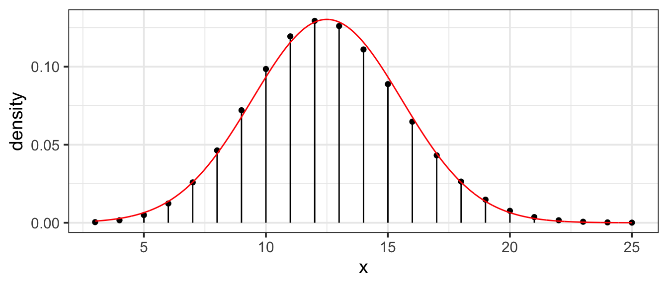
11.6.2.1 Normal approximation to Binomial
Binomial distributions are approximately normal as long as \(np\) and \(n(1-p)\) are both at least 10. Here is an example with \(n = 50\) and \(p = 0.25\) (so \(np = 12.5\)):
11.6.2.2 Normal approximation to Poisson
Poisson distributions become more and more like normal distributions as the rate increases.

Example 11.15 (Bad Luck at Roulette?) You have been playing a roulette game all night, betting on red, your lucky color. Altogether you have played n = 100 games and you know the probability of a random roll coming up red is 16 / 34. You’ve won only 42 games – you’re losing serious money. Are you unlucky? Has Red abandoned you?
If you have a calculator, you can find out approximately how unlucky you are. The setting is binomial, with n = 100 trials and p = 16/34. The mean and standard deviation of a binomial random variable are \(np\) and \(\sqrt{n p (1-p)}\), respectively; these formulas are ones that all skilled gamblers ought to know. For our situation, this works out to
\[ p = \frac{16}{34} = 0.471 \]
\[ \mathrm{mean} = n p = 100 \cdot 0.4706 = 47.1 \] \[ \mathrm{standard\ deviation} = \sqrt{n p (1-p)} = \sqrt{100 \cdot 0.4706 \cdot 0.5294} = 4.992 \]
The z-score of your performance is:
\[ z = \frac{42 - 47.1}{4.992} = -1.02 \]
It turns out that this binomial distribution is very similar to a normal distribution with the same mean and standard deviation. So the probability of doing this badly (or worse) is about 16% (the approximate normal percentile for a z-score of -1). Your performance isn’t good, but it’s not too surprising either.
When you get back to your hotel room, you can use your computer to do the exact calculation based on the binomial model. The probability of winning 42 or fewer games is 18.1%.

The outcome set goes by other names as well. It is conventionally called the sample space. This terminology can be confusing since it has little to do with the sort of sampling encountered in the collection of data nor with the sorts of spaces that vectors live in. If the outcome set conists of numbers (an important special case, called a random variable), then the outcome set is sometimes called the support of the random variable. For the most part, we’ll stick with outcome set since it is a clear description of what we mean.↩︎